Parallélisme : travaux dirigés et pratiques
- cours 1 : Introduction Générale
- cours 2 : Algorithmes et Métriques
- cours 3 : P-Threads et C++11 Threads
- cours 4 : OpenMP
- cours 5 : MPI
2. Algorithmes et Métriques
Dans ce chapitre nous nous intéressons à quelques algorithmes que l'on peut paralléliser. Certains sont trivialement parallélisables, d'autres demandent un peu plus de travail et de réflexion. Le but est de se familiariser avec les techniques liées au passage du séquentiel au parallèle.
2.1. Réduction
On considère un tableau de $n$ éléments et un opérateur associatif et commutatif $⊕$ doté d'un élément neutre $I$. A partir du tableau
$$ [ a_0, a_1, ..., a_{n-1} ] $$
on désire obtenir un unique résultat :
$$ a_0 ⊕ a_1 ⊕ ... ⊕ a_{n-1} $$
Si $⊕$ est l'addition alors la réduction permet d'obtenir la somme des éléments du tableau.
On peut appliquer cet algorithme avec d'autres opérateurs comme la multiplication, minimum, maximum.
Pour que l'algorithme soit parallélisable efficacement il suffit que l'opérateur $⊕$ dispose des propriétés d'associativité et de commutativité :
- commutativité : $a ⊕ b = b ⊕ a$
- associativité : $a ⊕ (b ⊕ c) = (a ⊕ b) ⊕ c$
2.1.1. code séquentiel
Voici le code séquentiel (et parallèle) en C++ de la réduction qui est facilement vectorisable :
- CODE
- sum_reduction.cpp
- // ==================================================================
- // Author: Jean-Michel RICHER
- // Email: jean-michel.richer@univ-angers.fr
- // Institution: LERIA, Faculty of Science
- // University of Angers, France
- // ==================================================================
- #include <iostream>
- #include <iomanip>
- using namespace std;
- /* ==================================================================
- * SUBPROGRAM
- *
- * float sum_reduction( float *t, int size );
- *
- * WHAT
- *
- * Perform sum of values of the array @param(t) of
- * @param(size) elements
- *
- * HOW
- *
- * Simply iterate and sum each value.
- *
- * PARAMETERS
- *
- * @paramdef(float, t) : array
- * @paramdef(int, size) : size of the array
- *
- * ==================================================================
- */
- float sum_reduction( float *t, int size ) {
- float total = 0.0;
- // OpenMP directive for parallelization
- #pragma omp parallel for reduction(+:total)
- for (int i = 0; i < size; ++i) {
- total += t[ i ];
- }
- return total;
- }
- /* ==================================================================
- * SUBPROGRAM
- *
- * int main(int argc, char *argv[])
- *
- * WHAT
- *
- * Main program
- *
- * PARAMETERS
- *
- * @paramdef(int,argc) : number of command line arguments
- * @paramdef(char **, argv) : command line arguments as C-strings
- *
- * ==================================================================
- */
- int main(int argc, char *argv[]) {
- // maximum number of values in the array
- const int MAX_VALUES = 10'000'000;
- // array of floats
- float *data;
- // allocate array
- data = new float [ MAX_VALUES ];
- // fill array
- for (int i=0; i <MAX_VALUES; ++i) {
- data[ i ] = 1.0;
- }
- // perform reduction as sum of values
- float sum = sum_reduction( data, MAX_VALUES );
- // print result
- cout << "sum=" << std::fixed << std::setprecision(2) << sum << endl;
- return EXIT_SUCCESS;
- }
Exercice 2.1
Compilez et exécutez le programme précédant avec en paramètre en ligne de commande :
- soit
1 pour la version séquentielle - soit
2 pour la version parallèle
mesurez et comparez les temps d'exécution en utilisant la commande qui suit avec les paramètres 1 ou 2 :
2.1.2. code parallèle
On dispose de $K$ processeurs et on répartit les indices à traiter entre les processeurs.
Pour la répartition des indices il existe deux possibilités à moins que les indices se répartissent équitablement :
- soit le dernier thread traite moins de valeurs que les autres
- soit le dernier thread traite plus de valeurs que les autres
2.1.2.a le dernier thread traite moins de valeurs que les autres
Chaque thread traite au plus $ μ_1 = (N + K -1) / K $ valeurs
| N | K | $μ_1$ | values |
| 100 | 2 | 50 | 50, 50 (=100) |
| 100 | 3 | 34 | 34, 34, 32 (=100) |
| 100 | 4 | 25 | 25, 25, 25, 25 (=100) |
| 100 | 5 | 20 | 20, 20, 20, 20, 20 (=100) |
| 100 | 6 | 17 | 17, 17, 17, 17, 17, 15 (=100) |
| 100 | 7 | 15 | 15, 15, 15, 15, 15, 15, 10 (=100) |
| 100 | 8 | 13 | 13, 13, 13, 13, 13, 13, 13, 9 (=100) |
| 101 | 2 | 51 | 51, 50 (=101) |
| 101 | 3 | 34 | 34, 34, 33 (=101) |
| 101 | 4 | 26 | 26, 26, 26, 23 (=101) |
| 101 | 5 | 21 | 21, 21, 21, 21, 17 (=101) |
| 101 | 6 | 17 | 17, 17, 17, 17, 17, 16 (=101) |
| 101 | 7 | 15 | 15, 15, 15, 15, 15, 15, 11 (=101) |
| 101 | 8 | 13 | 13, 13, 13, 13, 13, 13, 13, 10 (=101) |
| 102 | 2 | 51 | 51, 51 (=102) |
| 102 | 3 | 34 | 34, 34, 34 (=102) |
| 102 | 4 | 26 | 26, 26, 26, 24 (=102) |
| 102 | 5 | 21 | 21, 21, 21, 21, 18 (=102) |
| 102 | 6 | 17 | 17, 17, 17, 17, 17, 17 (=102) |
| 102 | 7 | 15 | 15, 15, 15, 15, 15, 15, 12 (=102) |
| 102 | 8 | 13 | 13, 13, 13, 13, 13, 13, 13, 11 (=102) |
| 103 | 2 | 52 | 52, 51 (=103) |
| 103 | 3 | 35 | 35, 35, 33 (=103) |
| 103 | 4 | 26 | 26, 26, 26, 25 (=103) |
| 103 | 5 | 21 | 21, 21, 21, 21, 19 (=103) |
| 103 | 6 | 18 | 18, 18, 18, 18, 18, 13 (=103) |
| 103 | 7 | 15 | 15, 15, 15, 15, 15, 15, 13 (=103) |
| 103 | 8 | 13 | 13, 13, 13, 13, 13, 13, 13, 12 (=103) |
- CODE
- repartition_v1.cpp
- // ==================================================================
- // Author: Jean-Michel RICHER
- // Email: jean-michel.richer@univ-angers.fr
- // Institution: LERIA, Faculty of Science
- // University of Angers, France
- // ==================================================================
- #include <iostream>
- #include <string>
- #include <vector>
- #include <numeric>
- using namespace std;
- /* ==================================================================
- * SUBPROGRAM
- *
- * void share_elements(int N, int K, vector<int>& velems);
- *
- * WHAT
- *
- * Distribute @param(N) elements over @param(K) processors
- *
- * HOW
- *
- * Assume that last processor will potentially have less
- * elements that others
- *
- * PARAMETERS
- *
- * @paramdef(int, N) : number of elements
- * @paramdef(int, K) : number of processors / process / threads
- * @paramdef(vector<int>&, velems) : vector that receives for each
- * processor the number of elements it will have to treat
- *
- * ==================================================================
- */
- void share_elements(int N, int K, vector<int>& velems) {
- int u_1, left = N;
- u_1 = (N + K - 1) / K;
- for (int k = 0; k < K-1; ++k) {
- velems.push_back( u_1 );
- left -= u_1;
- }
- velems.push_back( left );
- }
- /* ==================================================================
- * SUBPROGRAM
- *
- * int main(int argc, char *argv[])
- *
- * WHAT
- *
- * Main program
- *
- * PARAMETERS
- *
- * @paramdef(int,argc) : number of command line arguments
- * @paramdef(char **, argv) : command line arguments as C-strings
- *
- * ==================================================================
- */
- int main(int argc, char *argv[]) {
- // Number of elements, i.e. size of an array
- int N = 105;
- // Number of processors / process / threads
- int K = 6;
- if (argc > 1) N = atoi( argv[1] );
- if (argc > 2) K = atoi( argv[2] );
- vector<int> v_nbr_elements;
- share_elements( N, K, v_nbr_elements );
- cout << "-------------------" << endl;
- for (int k = 0; k < K; ++k) {
- cout << "k=" << k << ", #elements=" << v_nbr_elements[ k ] << endl;
- }
- int sum = accumulate( v_nbr_elements.begin(),
- v_nbr_elements.end(),
- 0);
- cout << "-------------------" << endl;
- cout << "sum=" << sum << endl;
- cout << "-------------------" << endl;
- return EXIT_SUCCESS;
- }
2.1.2.b le dernier thread traite plus de valeurs que les autres
Chaque thread traite au moins $ μ_2 = N / K $ valeurs
| N | K | $μ_2$ | values |
| 100 | 2 | 50 | 50, 50 (=100) |
| 100 | 3 | 33 | 33, 33, 34 (=100) |
| 100 | 4 | 25 | 25, 25, 25, 25 (=100) |
| 100 | 5 | 20 | 20, 20, 20, 20, 20 (=100) |
| 100 | 6 | 16 | 16, 16, 16, 16, 16, 20 (=100) |
| 100 | 7 | 14 | 14, 14, 14, 14, 14, 14, 16 (=100) |
| 100 | 8 | 12 | 12, 12, 12, 12, 12, 12, 12, 16 (=100) |
| 101 | 2 | 50 | 50, 51 (=101) |
| 101 | 3 | 33 | 33, 33, 35 (=101) |
| 101 | 4 | 25 | 25, 25, 25, 26 (=101) |
| 101 | 5 | 20 | 20, 20, 20, 20, 21 (=101) |
| 101 | 6 | 16 | 16, 16, 16, 16, 16, 21 (=101) |
| 101 | 7 | 14 | 14, 14, 14, 14, 14, 14, 17 (=101) |
| 101 | 8 | 12 | 12, 12, 12, 12, 12, 12, 12, 17 (=101) |
| 102 | 2 | 51 | 51, 51 (=102) |
| 102 | 3 | 34 | 34, 34, 34 (=102) |
| 102 | 4 | 25 | 25, 25, 25, 27 (=102) |
| 102 | 5 | 20 | 20, 20, 20, 20, 22 (=102) |
| 102 | 6 | 17 | 17, 17, 17, 17, 17, 17 (=102) |
| 102 | 7 | 14 | 14, 14, 14, 14, 14, 14, 18 (=102) |
| 102 | 8 | 12 | 12, 12, 12, 12, 12, 12, 12, 18 (=102) |
| 103 | 2 | 51 | 51, 52 (=103) |
| 103 | 3 | 34 | 34, 34, 35 (=103) |
| 103 | 4 | 25 | 25, 25, 25, 28 (=103) |
| 103 | 5 | 20 | 20, 20, 20, 20, 23 (=103) |
| 103 | 6 | 17 | 17, 17, 17, 17, 17, 18 (=103) |
| 103 | 7 | 14 | 14, 14, 14, 14, 14, 14, 19 (=103) |
| 103 | 8 | 12 | 12, 12, 12, 12, 12, 12, 12, 19 (=103) |
- CODE
- repartition_v2.cpp
- // ==================================================================
- // Author: Jean-Michel RICHER
- // Email: jean-michel.richer@univ-angers.fr
- // Institution: LERIA, Faculty of Science
- // University of Angers, France
- // ==================================================================
- #include <iostream>
- #include <string>
- #include <vector>
- #include <numeric>
- using namespace std;
- /* ==================================================================
- * SUBPROGRAM
- *
- * void share_elements(int N, int K, vector<int>& velems);
- *
- * WHAT
- *
- * Distribute @param(N) elements over @param(K) processors
- *
- * HOW
- *
- * Assume that last processor will potentially have more
- * elements that others
- *
- * PARAMETERS
- *
- * @paramdef(int, N) : number of elements
- * @paramdef(int, K) : number of processors / process / threads
- * @paramdef(vector<int>&, velems) : vector that receives for each
- * processor the number of elements it will have to treat
- *
- * ==================================================================
- */
- void share_elements(int N, int K, vector<int>& velems) {
- int u_2, left = N;
- u_2 = N / K;
- for (int k = 0; k < K-1; ++k) {
- velems.push_back( u_2 );
- left -= u_2;
- }
- velems.push_back( left );
- }
- /* ==================================================================
- * SUBPROGRAM
- *
- * int main(int argc, char *argv[])
- *
- * WHAT
- *
- * Main program
- *
- * PARAMETERS
- *
- * @paramdef(int,argc) : number of command line arguments
- * @paramdef(char **, argv) : command line arguments as C-strings
- *
- * ==================================================================
- */
- int main(int argc, char *argv[]) {
- // Number of elements, i.e. size of an array
- int N = 105;
- // Number of processors / process / threads
- int K = 6;
- if (argc > 1) N = atoi( argv[1] );
- if (argc > 2) K = atoi( argv[2] );
- vector<int> v_nbr_elements;
- share_elements( N, K, v_nbr_elements );
- cout << "-------------------" << endl;
- for (int k = 0; k < K; ++k) {
- cout << "k=" << k << ", #elements=" << v_nbr_elements[ k ] << endl;
- }
- int sum = accumulate( v_nbr_elements.begin(),
- v_nbr_elements.end(),
- 0);
- cout << "-------------------" << endl;
- cout << "sum=" << sum << endl;
- cout << "-------------------" << endl;
- return EXIT_SUCCESS;
- }
2.1.2.c répartition équitable
On répartit les $N$ éléments sur les $K$ threads, il reste alors $R = N - K (N/K)$ éléments que l'on assigne successivement à chaque thread :
| N | K | values |
| 100 | 2 | 50,50 |
| 100 | 3 | 34,33,33 |
| 100 | 4 | 25,25,25,25 |
| 100 | 5 | 20,20,20,20,20 |
| 100 | 6 | 17,17,17,17,16,16 |
| 100 | 7 | 15,15,14,14,14,14,14 |
- CODE
- repartition_v3.cpp
- // ==================================================================
- // Author: Jean-Michel RICHER
- // Email: jean-michel.richer@univ-angers.fr
- // Institution: LERIA, Faculty of Science
- // University of Angers, France
- // ==================================================================
- #include <iostream>
- #include <string>
- #include <vector>
- #include <numeric>
- using namespace std;
- /* ==================================================================
- * SUBPROGRAM
- *
- * void share_elements(int N, int K, vector<int>& velems);
- *
- * WHAT
- *
- * Distribute @param(N) elements over @param(K) processors
- *
- * HOW
- *
- * Assume that the number of elements is well distributed over
- * the processors
- *
- * PARAMETERS
- *
- * @paramdef(int, N) : number of elements
- * @paramdef(int, K) : number of processors / process / threads
- * @paramdef(vector<int>&, velems) : vector that receives for each
- * processor the number of elements it will have to treat
- *
- * ==================================================================
- */
- void share_elements(int N, int K, vector<int>& velems) {
- int u_2 = N / K, left = N;
- int k;
- for (k = 0; k < K; ++k) {
- velems.push_back( u_2 );
- left -= u_2;
- }
- k = 0;
- while (left != 0) {
- ++velems[ k ];
- --left;
- // here the '% K' is not necessary has there are left < K
- // elements to place
- k = (k + 1 ) % K;
- }
- }
- /* ==================================================================
- * SUBPROGRAM
- *
- * int main(int argc, char *argv[])
- *
- * WHAT
- *
- * Main program
- *
- * PARAMETERS
- *
- * @paramdef(int,argc) : number of command line arguments
- * @paramdef(char **, argv) : command line arguments as C-strings
- *
- * ==================================================================
- */
- int main(int argc, char *argv[]) {
- // Number of elements, i.e. size of an array
- int N = 105;
- // Number of processors / process / threads
- int K = 6;
- if (argc > 1) N = atoi( argv[1] );
- if (argc > 2) K = atoi( argv[2] );
- vector<int> v_nbr_elements;
- share_elements( N, K, v_nbr_elements );
- cout << "-------------------" << endl;
- for (int k = 0; k < K; ++k) {
- cout << "k=" << k << ", #elements=" << v_nbr_elements[ k ] << endl;
- }
- int sum = accumulate( v_nbr_elements.begin(),
- v_nbr_elements.end(),
- 0);
- cout << "-------------------" << endl;
- cout << "sum=" << sum << endl;
- cout << "-------------------" << endl;
- return EXIT_SUCCESS;
- }
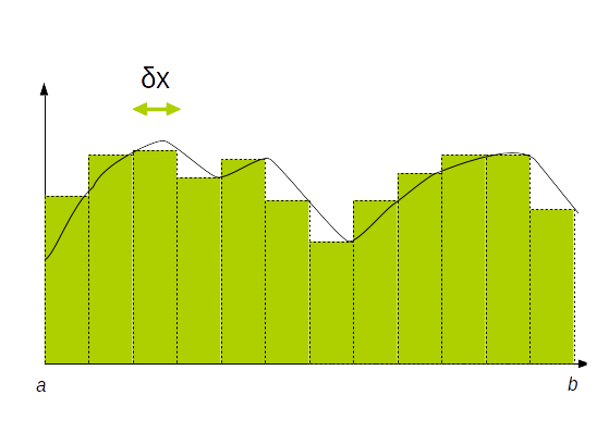
2.1.3. Application : calcul d'intégrale
Pour calculer l'intégrale d'une fonction $f(x)$ entre $a$ et $b$ on utilise la méthode des rectangles (ou des trapèzes si on désire une meilleure précision) qui consiste à décomposer l'intervalle $[a..b]$ en un ensemble de petits rectangles dont on va calculer l'aire.
Plus le nombre de rectangles est important plus la précision du résultat sera proche de la valeur réelle.
$$ ∫_a^b f(x)\, dx = ∑↙{i=1}↖N f(a + i × δx) × δx = δx × ∑↙{i=1}↖N f(a + i × δx) $$
avec
$$ δx = {(b - a)} / N $$
2.1.3.a code séquentiel
Le code en C++ du calcul de l'intégrale de $f(x) = x^2$ entre 0 et 3.0 est le suivant :
- CODE
- integrale.cpp
- // ==================================================================
- // Author: Jean-Michel RICHER
- // Email: jean-michel.richer@univ-angers.fr
- // Institution: LERIA, Faculty of Science
- // University of Angers, France
- // ==================================================================
- // Compute integral of function f(x) = x^2 between X_0 and X_1
- // using area of rectangles
- #include <iostream>
- #include <cmath>
- using namespace std;
- typedef double real;
- real X_0 = 1.0;
- real X_1 = 3.0;
- int STEPS = 1'000'000;
- /* ==================================================================
- * SUBPROGRAM
- *
- * real f(real x ;
- *
- * WHAT
- *
- * Function to integrate
- *
- *
- * PARAMETERS
- *
- * @paramdef(real, x) : abscissa
- *
- * ==================================================================
- */
- real f( real x ) {
- return x * x;
- }
- /* ==================================================================
- * SUBPROGRAM
- *
- * real integrate(real x_0, real x_1, int steps)
- *
- * WHAT
- *
- * Use the sum of rectangles under the function
- *
- * HOW
- *
- * We compute the sum of (x_1 - x_0) / steps rectangles
- *
- * PARAMETERS
- *
- * @paramdef(real, x_0) : lower bound
- * @paramdef(real, x_1) : upper bound
- * @paramdef(int, steps) : number of rectangles to use
- *
- * RETURN VALUE
- *
- * @return(real) the sum of all rectangles that compose the
- * integral
- *
- * ==================================================================
- */
- real integrate(real x_0, real x_1, int steps) {
- real dx, local;
- real delta_x = (x_1 - x_0) / steps;
- real area = 0;
- for (int i = 1; i <= steps; ++i) {
- area += f(x_0 + i * delta_x);
- }
- return delta_x * area;
- }
- /* ==================================================================
- * SUBPROGRAM
- *
- * int main(int argc, char *argv[])
- *
- * WHAT
- *
- * Main program
- *
- * PARAMETERS
- *
- * @paramdef(int,argc) : number of command line arguments
- * @paramdef(char **, argv) : command line arguments as C-strings
- *
- * ==================================================================
- */
- int main() {
- cout << "integrate(" << X_0 << ", " << X_1 << ")=" << integrate(X_0, X_1, STEPS) << endl;
- return EXIT_SUCCESS;
- }
2.1.3.b code parallèle
Si on dispose de $K$ processeurs ou machines, on répartit les calculs sur $K$ machines
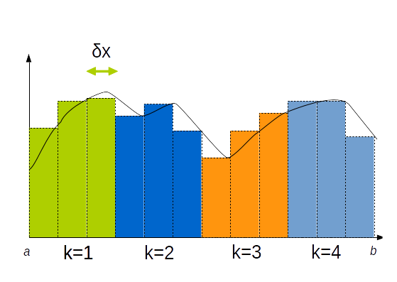
Chaque $P_k, k ∊ [1..K]$ calcule en moyenne $γ = N/K$ valeurs :
- CODE
- integrale_omp.cpp
- // ==================================================================
- // Author: Jean-Michel RICHER
- // Email: jean-michel.richer@univ-angers.fr
- // Institution: LERIA, Faculty of Science
- // University of Angers, France
- // ==================================================================
- // Compute integral of function f(x) = x^2 between X_0 and X_1
- // using area of rectangles
- #include <iostream>
- #include <cmath>
- using namespace std;
- typedef double real;
- real X_0 = 1.0;
- real X_1 = 3.0;
- int STEPS = 1'000'000;
- /* ==================================================================
- * SUBPROGRAM
- *
- * real f(real x ;
- *
- * WHAT
- *
- * Function to integrate
- *
- *
- * PARAMETERS
- *
- * @paramdef(real, x) : abscissa
- *
- * ==================================================================
- */real f(real x ) {
- return x * x;
- }
- /* ==================================================================
- * SUBPROGRAM
- *
- * real integrate(real x_0, real x_1, int steps)
- *
- * WHAT
- *
- * Use the sum of rectangles under the function
- *
- * HOW
- *
- * We compute the sum of (x_1 - x_0) / steps rectangles
- *
- * PARAMETERS
- *
- * @paramdef(real, x_0) : lower bound
- * @paramdef(real, x_1) : upper bound
- * @paramdef(int, steps) : number of rectangles to use
- *
- * RETURN VALUE
- *
- * @return(real) the sum of all rectangles that compose the
- * integral
- *
- * ==================================================================
- */
- real integrate(real x_0, real x_1, int steps) {
- real dx, local;
- real delta_x = (x_1 - x_0) / steps;
- real area = 0;
- #pragma omp parallel for reduction(+:area)
- for (int i = 1; i <= steps; ++i) {
- area += f(x_0 + i * delta_x);
- }
- return delta_x * area;
- }
- /* ==================================================================
- * SUBPROGRAM
- *
- * int main(int argc, char *argv[])
- *
- * WHAT
- *
- * Main program
- *
- * PARAMETERS
- *
- * @paramdef(int,argc) : number of command line arguments
- * @paramdef(char **, argv) : command line arguments as C-strings
- *
- * ==================================================================
- */
- int main() {
- cout << "integrate(" << X_0 << ", " << X_1 << ")=" << integrate(X_0, X_1, STEPS) << endl;
- return EXIT_SUCCESS;
- }
2.2. courbe de Julia
Les courbes ou ensembles de Julia, du mathématicien français Gaston Julia (1893 à 1978) ou ensembles de Mandelbrot du mathématicien Benoît Mandelbrot (1924-2010) sont un bon exemple d'application du parallélisme.
Etant donné un nombre complexe $z_0$ qui correspond à un point dans le plan, on associe la suite : $z_{n+1} = z_n^2 + c$, où $c$ est une constante complexe.
Le plan est alors partagé entre :
- l'ensemble des points pour lesquels la suite est bornée (qualifiés de prisonniers de $f$)
- les autres points étant les fugitifs
L'ensemble de Julia associé à $z_n$ est alors la frontière commune de ces deux ensembles, en fait, la ligne de démarcation entre les prisonniers et les fugitifs.
- CODE
- julia.cpp
- #include <iostream>
- #include <complex>
- using namespace std;
- double X_MIN = -1.0;
- double X_MAX = 1.0;
- double Y_MIN = -1.0;
- double Y_MAX = 1.0;
- double X_SIZE = X_MAX - X_MIN;
- double Y_SIZE = Y_MAX - Y_MIN;
- const int WIDTH = 100;
- const int HEIGHT = 100;
- int ITERATIONS = 1000;
- complex<double> c( 0.3, 0.5 );
- double PRISONERS_LIMIT = 4.0;
- char *jset;
- /**
- * check if function converge or not
- */
- bool is_prisoner(complex<double> z_0) {
- complex<double> z = z_0;
- int i = 0;
- while ((std::norm(z) < PRISONERS_LIMIT) and (i < ITERATIONS)) {
- z = z * z + c;
- i = i + 1;
- }
- return i >= ITERATIONS;
- }
- // -----------------------------
- //
- // -----------------------------
- void julia_set() {
- complex<double> z_0;
- for (int y = 0; y < HEIGHT; ++y) {
- for (int x = 0; x < WIDTH; ++x) {
- z_0 = complex<double>(X_MIN + ((double)x) / WIDTH * X_SIZE,
- Y_MIN + ((double)y) / HEIGHT * Y_SIZE );
- if (is_prisoner(z_0)) {
- jset[y * WIDTH + x] = 'X';
- } else {
- jset[y * WIDTH + x] = '.';
- }
- }
- }
- }
- void print() {
- for (int y = 0; y < HEIGHT; ++y) {
- for (int x = 0; x < WIDTH; ++x) {
- cout << jset[ y * WIDTH + x ];
- }
- cout << endl;
- }
- }
- // -----------------------------
- // program
- // -----------------------------
- int main(int argc, char *argv[]) {
- double factor = 1.0;
- if (argc > 1) factor = atof( argv[1] );
- X_MIN *= factor;
- X_MAX *= factor;
- Y_MIN *= factor;
- Y_MAX *= factor;
- X_SIZE = X_MAX - X_MIN;
- Y_SIZE = Y_MAX - Y_MIN;
- jset = new char [ HEIGHT * WIDTH ];
- julia_set();
- cout << "<html><body><pre>" << endl;
- print();
- cout << "</pre></body></html>" << endl;
- return EXIT_SUCCESS;
- }
Exercice 2.2
➊ Créer un programme qui permet de tester une méthode séquentielle et la comparer à une méthode parallèle en faisant évoluer le nombre de threads de 2 à 16 par pas de 2. En utilisera getopt afin de fournir des paramètres au programme :
- -v : mode verbeux pour afficher le résultat
- -w entier : pour définir la largeur de l'image en pixels
- -h entier : pour définir la hauteur de l'image en pixels
- -m entier : la méthode utilisée 1=séquentiel, 2=parallèle
➋ Créer un script
1 22.10
2 11.01
4 6.89
6 4.87
8 4.12
10 3.40
12 2.83
14 2.75
16 2.80
➌ Créer un script python
- le nombre de threads
- le temps en secondes
- l'accélération réelle
- l'accélération théorique selon Amdhal
- la métrique de Karp-flatt
Par exemple, pour les données précédentes on voudrait obtenir quelque chose comme :
\$ python3 exploit_results.py julia_results.txt
=============================================================
Analyse de la performance de l'application
Fraction parallèle (Par) utilisée pour Amdahl: 0.99
=============================================================
Threads  | Temps (s)   | Acc Réel. | Acc Amdahl | Karp-Flatt
-------------------------------------------------------------
1        |  22.1000    |  1.0000   |  1.0000    | -1.0000
2        |  11.0100    |  2.0073   |  1.9802    | -0.0036
4        |   6.8900    |  3.2075   |  3.8835    |  0.0824
6        |   4.8700    |  4.5380   |  5.7143    |  0.0644
8        |   4.1200    |  5.3641   |  7.4766    |  0.0702
10       |   3.4000    |  6.5000   |  9.1743    |  0.0598
12       |   2.8300    |  7.8092   | 10.8108    |  0.0488
14       |   2.7500    |  8.0364   | 12.3894    |  0.0571
16       |   2.8000    |  7.8929   | 13.9130    |  0.0685
Dans cet exemple, la métrique de Karp-flatt ($e$) est la plus faible pour un nombre de threads égal à 12, ce qui correspond aux 12 threads d'un AMD Ryzen 5 9600X.
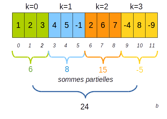
2.3. Scan
2.3.1. principe
L'algorithme de scan (aussi qualifié de prefix sum, cumulative sum, inclusive scan et exclusive scan) possède de nombreuses applications en informatique. Il consiste étant donnée une séquence de nombres $[a_0, a_1, ..., a_{n-1}]$ et un opérateur binaire associatif $⊕$ doté d'un élément neutre $I$, à calculer une deuxième séquence :
- exclusive scan : $[I, a_0, a_0 ⊕ a_1, ... , a_0 ⊕ a_1 + ... + a_{n-2} ]$
- inclusive scan : $[a_0, a_0 ⊕ a_1, ... , a_0 ⊕ a_1 + ... + a_{n-1} ]$
Vous trouverez plusieurs applications sur le site suivant : toves.org (voir notamment la section 3.3. Adding big integers)
Voici une première version séquentielle des algorithmes :
- CODE
- scan.cpp
- #include <iostream>
- #include <vector>
- using namespace std;
- void sequential_inclusive_scan( vector<int>& x ) {
- for (int i = 1; i < static_cast<int>(x.size()); ++i) {
- x[ i ] += x[ i-1 ];
- }
- }
- void sequential_exclusive_scan( vector<int>& x ) {
- int previous = x[0];
- x[0] = 0;
- for (int i = 1; i < static_cast<int>(x.size()); ++i) {
- int current = x[ i ];
- x[ i ] = x[ i-1 ] + previous;
- previous = current;
- }
- }
- int main() {
- vector<int> x1 = { 1, 3, 5, 7, 9, 20 };
- vector<int> x2 = { 1, 3, 5, 7, 9, 20 };
- sequential_inclusive_scan( x1 );
- cout << "inclusive sacn=";
- for (auto x : x1) cout << x << " ";
- cout << endl;
- sequential_exclusive_scan( x2 );
- cout << "exclusive sacn=";
- for (auto x : x2) cout << x << " ";
- cout << endl;
- return EXIT_SUCCESS;
- }
Par exemple avec la séquence [1, 3, 5, 7, 9] et l'opérateur d'addition on obtient :
- exclusive scan : [0, 1, 4, 9, 16]
- inclusive scan : [1, 4, 9, 16, 25]
La complexité de cet algorithme est en $O(n)$
Malheureusement ces deux sous-programmes ne sont pas parallélisables directement.
On s'interessera par la suite au scan inclusif.
2.3.2. Versions parallèles
2.3.2.a un premier algorithme naïf
Un premier algorithme parallèle peut être exhibé mais il n'est pas très efficace : il repose sur l'utilisation de deux tableaux qui sont utilisés successivement en entrée et en sortie
- // ==================================================================
- // Author: Jean-Michel RICHER
- // Email: jean-michel.richer@univ-angers.fr
- // Institution: LERIA, Faculty of Science
- // University of Angers, France
- // ==================================================================
- #include <iostream>
- #include <vector>
- #include <cmath>
- #include <numeric>
- using namespace std;
- /**
- * Send vector contents to output stream
- *
- */
- template<class T>
- ostream& operator<<( ostream& out, vector<T>& v) {
- for (auto x : v) out << x << " ";
- return out;
- }
- /* ==================================================================
- * SUBPROGRAM
- *
- * vector<int>& sequential_inclusive_scan( vector<int> &x,
- * vector<int>& y );
- *
- * WHAT
- *
- * Perform inclusive scan in parallel with two buffers
- *
- * HOW
- *
- * We use a log2(n) algorithm, however, for the result to be correct
- * we need to add 1 to log2(n) if n > 2^log2(n). For example, if n,
- * the size of the input vector @param(in) is equal to 8, then
- * @var(log2n) = 3. But if n == 9, @var(log2n) should be set to 4.
- *
- * At each step we compute 2^(d-1) that we call @var(shift) where
- * @var(d) ranges from 1 to @var(log2n).
- *
- * We copy the data from the input vector @param(in) from 0 to
- * @var(shift)-1.
- * We add to the other elements of the input vector, the elements
- * that are shifted from @var(shift).
- *
- *
- * PARAMETERS
- *
- * @paramdef(vector<int>&, in) : input vector of data
- * @paramdef(vector<int>&, out) : vector used for calculations
- *
- *
- * RETURN VALUE
- * @return(vector<int>&) reference to last modified vector
- *
- * ==================================================================
- */
- vector<int>& parallel_naive_inclusive_scan( vector<int> &x, vector<int>& y ) {
- vector<int> &in = x;
- vector<int> &out = y;
- int n = static_cast<int>( x.size() );
- // if use this, then we won't have the correct result if n
- // is not a power of 2
- //int log2n = round( log2( n ) );
- int log2n = 32 - __builtin_clz( n ) - 1;
- if (__builtin_popcount( n ) > 1) ++log2n;
- for (int d = 1; d <= log2n; ++d) {
- int shift = 1 << (d-1);
- // copy values under shift
- #pragma omp parallel for
- for (int i = 0; i < shift; ++i) {
- out[ i ] = in [ i ];
- }
- // add values over shift
- #pragma omp parallel for
- for (int i = shift; i < n; ++i) {
- out[ i ] = in[ i ] + in[ i - shift ];
- }
- swap( in, out );
- }
- return in;
- }
- /* ==================================================================
- * SUBPROGRAM
- *
- * int main(int argc, char *argv[])
- *
- * WHAT
- *
- * Main program
- *
- * PARAMETERS
- *
- * @paramdef(int,argc) : number of command line arguments
- * @paramdef(char **, argv) : command line arguments as C-strings
- *
- * ==================================================================
- */
- int main(int argc, char *argv[]) {
- vector<int> x1;
- vector<int> x2;
- int n = 8;
- if (argc > 1) n = atoi( argv[1] );
- x1.resize( n );
- x2.resize( n );
- //iota(x1.begin(), x1.end(), 1);
- for (auto i = x1.begin(); i != x1.end(); ++i) *i = 1;
- cout << "initial data=" << x1 << endl;
- vector<int>& r = sequential_inclusive_scan( x1, x2 );
- cout << "inclusive scan=" << r << endl;
- return EXIT_SUCCESS;
- }
La complexité de cet algorithme est en $O(n × \log_2(n))$, elle augmente donc la complexité de l'algorithme séquentiel par un facteur $\log_2(n)$.
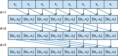
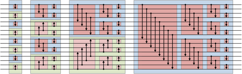
2.3.2.b un second algorithme efficace
L'idée est d'utiliser un parcours sous forme d'arbre. On utilise deux phases appelées sweep (balayage) :
- la phase ascendante (up-sweep phase) correspond à un parcours des feuilles vers la racine : on calcule des sommes partielles pour chaque noeud interne. Il s'agit en fait d'un algorithme de réduction
- la phase descendante (down-sweep phase) correspond à un parcours de la racine vers les feuilles
Ce genre d'algorithme se révèle moins efficace que l'algorithme séquentiel mais peut être intéressant sur des architectures de type GPU.
|

|
a) phase up-sweep
la phase de balayage vers la haut consiste à parcourir le tableau sous la forme d'un arbre binaire en calculant des sommes partielles :
- on commence au niveau $d = 1$ avec les éléments d'indice modulo 2
- puis modulo 4 au niveau suivant $d = 2$
- jusqu'à atteindre la taille du tableau : $n = 8 = 2^{d = 3}$
Voici une première version avec $d ∈ [1..log_2(n)]$ :
// up-sweep - version 1
for d in [1 : log2(n)] do

        var int shift = 2^d

        for i in [1 : n] do
                if int(modulo(i, shift)) = 0 then
                        a[i] = a[i] + a[i - shift / 2]
                endif
        endfor

endfor
Cependant ajouter un if dans le code n'apporte rien pour la parallélisation. Voici donc une autre version de l'up-sweep qui sera plus simplement parallélisable:
// up-sweep - version 2 - scan inclusif
var int start = 0, shift = 2

for d in [1 : log2(n)] do

        for i in parallel [start : n-1 : shift] do
                a[i + shift / 2] += a[i]
        endfor

        start = shift - 1
        shift = 2 * shift

endfor
b) phase down-sweep
Dans le cadre du scan inclusif il faut procéder ainsi :
// down sweep - inclusive scan

var int start = (n /2) - 1, shift = 1 << (log2(n)-1)

for d in [log2(n): 1 : -1] do

        for i in parallel [start : n-2 : 2 * shift  ] do
            a[i + shift] += a[i];
        endfor

        start -= shift
        shift /= 2

endfor
Exercice 2.3
Créer un programme qui permet de tester les différentes méthodes de scan inclusif.
- sequential_inclusive_scan
- parallel_naive_inclusive_scan
- sequential_sweep_inclusive_scan
- parallel_sweep_inclusive_scan
Pour chaque méthode, répétez 10000 fois la création d'un vecteur de 65536 double comprenant les valeurs de 1 à 65536 et le calcul du scan.
Créer un script bash qui permet de tester les méthodes séquentielles ou parallèles.
Au final la parallélisation de cet algorithme n'est pas efficace :
| Méthode | Complexité |
| Séquentiel | O(n) |
| Parallèle naïf | O(n log2(n)) |
| parallèle balayage (sweep) | O(n) |
| Méthode | Temps (s) |
| séquentiel (1 thread) | 0.55 |
| parallèle naïf (12 threads) | 2.36 |
| balayage séquentiel (1 thread) | 0.68 |
| balayage parallèle (12 threads) | 0.59 |
2.4. Les algorithmes de tri
Il est important de choisir des algorithmes qui seront parallélisables naturellement. Par exemple le tri à bulle est difficilement parallélisable.
Nous verrons trois types de tri :
- tri pair-impair (odd-even)
- tri fusion (merge)
- tri bitonique (bitonic)
2.4.1. Tri pair-impair (odd-even sort)
Le principe du tri pair-impair est de comparer les couples/paires d'éléments d'un tableau.
- dans un premier temps on compare les couples d'indices pairs (0, 2, 4, ...), en d'autre termes on compare t[0] avec t[1], puis t[2] avec t[3], etc...
- puis dans un second temps les couples d'indices impaires (1, 3, 5, ...), en d'autres termes on compare t1] avec t[2], puis t[3] avec t[4], etc...
On recomence jusqu'à ce que le tableau soit trié.
Voici un exemple avec un tableau dont les valeurs sont trié en ordre inverse. On peut voir que les valeurs 5 et 12 apparaissent sur les diagonales lors des différentes étapes de tri.
| étape/indice | 0 | 1 | 2 | 3 | 4 | 5 | 6 | 7 |
| initial | 12 | 11 | 10 | 9 | 8 | 7 | 6 | 5 |
| 1.pair | 11 | 12 | 9 | 10 | 7 | 8 | 5 | 6 |
| 1.impair | 11 | 9 | 12 | 7 | 10 | 5 | 8 | 6 |
| 2.pair | 9 | 11 | 7 | 12 | 5 | 10 | 6 | 8 |
| 2.impair | 9 | 7 | 11 | 5 | 12 | 6 | 10 | 8 |
| 3.pair | 7 | 9 | 5 | 11 | 6 | 12 | 8 | 10 |
| 3.impair | 7 | 5 | 9 | 6 | 11 | 8 | 12 | 10 |
| 4.pair | 5 | 7 | 6 | 9 | 8 | 11 | 10 | 12 |
| 4.impair | 5 | 6 | 7 | 8 | 9 | 10 | 11 | 12 |
- CODE
- odd_even_sort.ezl
- procedure odd_even_sort(t is array of integer)
- // tells whether array is sorted or not
- variable is_sorted is boolean
- do
- is_sorted = true
- // even index sort
- for i in range(0,N-1) step 2 do
- if t[i] > t[i+1] then
- swap(t[i], t[i+1])
- is_sorted = false
- end if
- end for
- // odd index sort
- for i in range(1, N-2) step 2 do
- if t[i] > t[i+1] then
- swap(t[i], t[i+1])
- is_sorted = false
- end if
- end for
- while (not is_sorted)
- end procedure
GeSHi Error: GeSHi could not find the language ezl (using path /home/jeanmichel.richer/public_html/php-geshi/geshi/) (code 2)
2.4.2. Tri fusion (merge sort)
Le tri fusion consiste :
- dans une première phase : à décomposer le tableau (split) en tableaux plus petits, on divise le tableau en 2 à chaque étape ce qui conduit à une décomposition arborescente en $log_2(n)$. Lorsque le tableau a une taille de deux éléments on trie les deux éléments du tableau
- dans une deuxième phase : à fusionner (merge) deux tableaux triés adjacents
- CODE
- merge_sort.cpp
- #include <iostream>
- #include <cstring> // for memcpy
- using namespace std;
- /* ==================================================================
- * SUBPROGRAM
- *
- * void merge<T>(T *t, int a, int m, int b)
- *
- * WHAT
- * Merge two consecutive sorted subarrays into one from indices
- * [a,m-1] to [m,b-1].
- *
- * HOW
- * We use a temporary array of size b-a called tmp to store
- * the result and then we copy it to its destination in t
- * starting at index a.
- *
- * PARAMETERS
- *
- * @param t array of generic type T
- * @param a index at the beginning of the array
- * @param m index on the middle of the array
- * @param b index at the end of the array
- *
- * ==================================================================
- */
- template<class T>
- void merge(T *t, int a, int m, int b) {
- // size of temporary array
- int tmp_size = b-a;
- // create temporary array to store sorted data
- T *tmp = new T [ tmp_size ];
- // indices to go through subarrays
- int i1, i2, l1, l2, k;
- i1 = a;
- l1 = m;
- i2 = m;
- l2 = b;
- k = 0;
- while ((i1 < l1) && (i2 < l2)) {
- if (t[i1] < t[i2]) {
- tmp[k++] = t[i1++];
- } else if (t[i2] < t[i1]) {
- tmp[k++] = t[i2++];
- } else {
- tmp[k++] = t[i1++];
- tmp[k++] = t[i2++];
- }
- }
- while (i1 < l1) {
- tmp[k++] = t[i1++];
- }
- while (i2 < l2) {
- tmp[k++] = t[i2++];
- }
- memcpy( &t[a], tmp, sizeof(T) * tmp_size );
- delete [] tmp;
- }
- /* ==================================================================
- * SUBPROGRAM
- *
- * void split(T *t, int a, int b);
- *
- * WHAT
- *
- * Recursively divide an array into two subarrays and then sort
- * each subarray and merge the two sorted subarrays.
- *
- * HOW
- * We divide the initial array from index a to b-1 into two
- * subarrays in the middle, i.e (b+a)/2. Note that we don't
- * really divide the array, but rather use the indices to mark
- * the begining and end of the array.
- * If the array is of size 1, we stop and go up one level.
- * If the array is of size 2, we sort the two values
- * If the array is of size > 2 then we recursively divide the
- * array in two.
- *
- * PARAMETERS
- *
- * @param t array to sort
- * @param a index at the beginning of the array
- * @param b index at the end of the array
- *
- * ==================================================================
- */
- template<class T>
- void split(T *t, int a, int b) {
- if ((b - a) <= 2) {
- if ((b - a) == 2) {
- if (t[a] > t[a+1]) {
- swap(t[a], t[a+1]);
- }
- }
- } else {
- int middle = (b+a)/2;
- split(t, a, middle);
- split(t, middle, b);
- merge(t, a, middle, b);
- }
- }
- /* ==================================================================
- * SUBPROGRAM
- *
- * merge_sort(T *t, int size);
- *
- * WHAT
- *
- * Perform merge sort on an array @param(t) of size @param(size)
- *
- *
- */
- template<class T>
- void merge_sort(T *t, int size) {
- split(t, 0, size);
- }
- /**
- * Programme principal
- */
- int main() {
- int size = 17;
- int *tab = new int [ size ];
- for (int i=0; i<size; ++i) tab[i] = size-i;
- merge_sort(tab, size);
- for (int i=0; i<size; ++i) cout << tab[i] << " ";
- cout << endl;
- return EXIT_SUCCESS;
- }
2.4.3. Tri bitonique (bitonic sort)
Voir l'article Tri bitonique de Wikipédia en français.
Exemple des comparaisons à réaliser (image issue de Wikipedia)
Le tableau doit avoir une taille égale à une puissance de 2.
// note that the array must have a size equal to a power of 2
var int dim is integer = 5
var array arr[0..2^dim-1]

proc bitonic_sort(array& t)

	var int log2_n = log2(size(t))

	for i in [0 : log2_n - 1] do
		for j in [0 : i] do
			compare(t, i, j, size(t))
		endfor
	endfor

end

proc compare(array& t, int p, q, size) {

	var int d  = 1 << (p-q)
	var bool up

	for i in [0 : size-1] do
		if ((i >> p) & 2) = 0 then
			up = true
		else
			up = false
		endif

		if (i & d) = 0 then
			if (t[i] > t[i + d]) = up then
				swap(t[i], t[i + d])
			endif
		endif
	endfor

end
2.5. Métriques : accélération, efficacité, loi de Amdhal
Voir ce document pour de plus amples explications.
2.5.1. Amélioration
Pour comparer deux implantations (implantation de REFérence et OPTimisée), on peut définir trois valeurs
- le facteur d'amélioration ou accélération (speedup): $$acc = T_{REF}/T_{OPT}$$ qui sera supérieur à 1 si la version OPTimisée est effectivement plus efficace que la version de REFérence
- le pourcentage d'amélioration : $$pct = ({T_{OPT} - T_{REF}})/T_{REF} × 100$$ qui sera négatif si la version OPTimisée est effectivement plus efficace que la version de REFérence
- l'efficacité $E$ est le rapport entre l'accélération et le nombre de processeurs $$E(K) = {acc}/{K}$$
| $T_{OPT}$ | 100 | 90 | 80 | 70 | 60 | 50 | 40 | 30 | 20 | 10 |
| accélération $(acc)$ | 1.00 | 1.11 | 1.25 | 1.43 | 1.67 | 2.00 | 2.50 | 3.33 | 5.00 | 10.00 |
| pourcentage $(pct)$ | 0% | -10% | -20% | -30% | -40% | -50% | -60% | -70% | -80% | -90% |
2.5.2. Loi de Amdahl
L'application de la loi de Amdahl (1967) en calcul parallèle permet de prédire l'accélération théorique que l'on peut espérer obtenir en utilisant plusieurs processeurs.
Cette loi peut être vue come un outil d'aide à la décision : connaissant le pourcentage de code parallélisable, on peut déterminer combien de processeurs/coeurs apporteront un gain maximal ou s'il est intéressant de passer de 2 à 4, de 4 à 8 processeurs pour diminuer significativement le temps de calcul.
Soit un programme qui s'exécute en $T_1$ secondes et soient $Seq$ et $Par$ respectivement le pourcentage de temps passé en séquentiel et en parallèle, alors le temps d'exécution par un seul processeur est défini par:
$$T_1 = Seq × T_1 + Par × T_1 = (1 - Par) × T_1 + Par × T_1 $$sachant que $Par + Seq = 1$. Par exemple si $Par=0.92$ alors 92% du temps est passé dans la section de code parallèle.
Si on utilise $K$ processeurs alors seule la partie parallèle en bénéficie. Le temps d'exécution $T_K$ pour $K$ processeurs est défini par : $$ T_K = Seq × T_1 + Par × T_1 / K $$
L'accélération pour $K$ processeurs est donnée par $acc = T_1 / T_K$ est alors :
$$ {T_1}/{T_K} = {(1 - Par) × T_1 + Par × T_1}/{(1 - Par) × T_1 + Par × T_1 / K} = 1 / {1 - Par + {Par}/ K} = 1 / {Seq + {1 - Seq}/ K} = 1/{Seq + {Par}/{K}} $$| $K$ | $Acc$ | % | $Δ$ % |
| 2 | 1.85 | -46 | 46 |
| 4 | 3.23 | -69 | 23 |
| 8 | 5.13 | -80 | 11 |
| 10 | 5.81 | -83 | 3 |
| 12 | 6.38 | -84 | 1 |
| 20 | 7.94 | -87 | 3 |
Notons que plus $Par$ est proche de 1, plus $acc$ est grand quand $K$ augmente, cf. l'image ci-dessous où $R=acc$ et $S=K$ le nombre de processeurs.
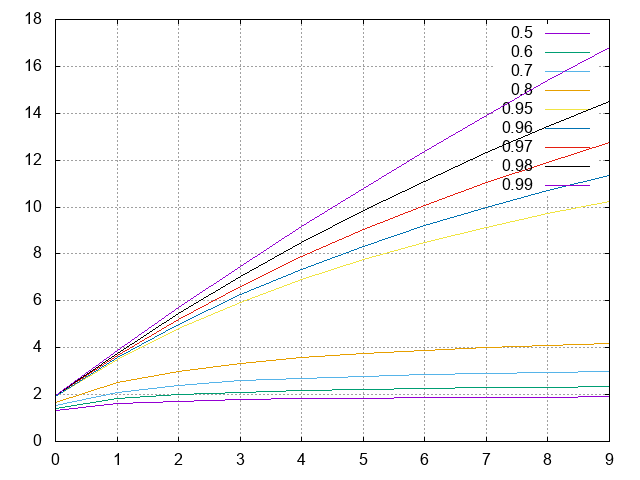
| K \ Par | 0.5 | 0.6 | 0.7 | 0.8 | 0.9 | 0.92 | 0.95 | 0.99 |
|---|---|---|---|---|---|---|---|---|
| 2 | 1.33 | 1.43 | 1.54 | 1.67 | 1.82 | 1.85 | 1.90 | 1.98 |
| 4 | 1.60 | 1.82 | 2.11 | 2.50 | 3.08 | 3.23 | 3.48 | 3.88 |
| 8 | 1.78 | 2.11 | 2.58 | 3.33 | 4.71 | 5.13 | 5.93 | 7.48 |
| 10 | 1.82 | 2.17 | 2.70 | 3.57 | 5.26 | 5.81 | 6.90 | 9.17 |
| 12 | 1.85 | 2.22 | 2.79 | 3.75 | 5.71 | 6.38 | 7.74 | 10.81 |
| 16 | 1.88 | 2.29 | 2.91 | 4.00 | 6.40 | 7.27 | 9.14 | 13.91 |
| 20 | 1.90 | 2.33 | 2.99 | 4.17 | 6.90 | 7.94 | 10.26 | 16.81 |
| 32 | 1.94 | 2.39 | 3.11 | 4.44 | 7.80 | 9.20 | 12.55 | 24.43 |
| 64 | 1.97 | 2.44 | 3.22 | 4.71 | 8.77 | 10.60 | 15.42 | 39.26 |
| 128 | 1.98 | 2.47 | 3.27 | 4.85 | 9.34 | 11.47 | 17.41 | 56.39 |
| 256 | 1.99 | 2.49 | 3.30 | 4.92 | 9.66 | 11.96 | 18.62 | 72.11 |
Par exemple avec 99% du temps d'exécution parallélisable, on peut diviser le temps d'exécution par un facteur 16.81 lorsque l'on utilise 20 threads/processeurs.
Attention cependant, dans certains cas la limite théorique peut ne pas être atteinte car la taille des données possède une influence sur le nombre de threads (exemple Maximum de Parcimonie $Par = 0.92$ limite atteinte pour $K=10$ à $12$)
2.5.3. Loi de Gustafson
La loi de Amdhal concerne l'accélération à travail ou charge constante. La loi de Gustafson prédit l’accélération théorique maximale obtenue en n'imposant pas que la taille du travail soit fixe.
D'après Wikipédia : Plus le nombre de données traitées en parallèles est grand, plus l’utilisation d'un grand nombre de processeurs est efficace. Mais surtout, il n'y a pas de limite théorique à l'accélération : on peut mettre autant de données que l'on veut, celles-ci sont toutes traitées par un processeur simultanément et le temps mis pour traiter s données sur s processeurs sera identique au temps mis pour traiter une donnée sur un seul processeur. Aucune limite n'existe concernant la quantité de données traitables simultanément, et donc au gain que l'on peut obtenir.
Elle traduit le fait que l'on peut traiter plus de données dans le même temps en augmentant le nombre de processeurs.
$$acc = Seq + K × Par = K + Seq × (1 - K)$$
| K / Par | 0.5 | 0.6 | 0.7 | 0.8 | 0.9 | 0.92 | 0.95 | 0.99 |
|---|---|---|---|---|---|---|---|---|
| 2 | 1.50 | 1.60 | 1.70 | 1.80 | 1.90 | 1.92 | 1.95 | 1.99 |
| 4 | 2.50 | 2.80 | 3.10 | 3.40 | 3.70 | 3.76 | 3.85 | 3.97 |
| 8 | 4.50 | 5.20 | 5.90 | 6.60 | 7.30 | 7.44 | 7.65 | 7.93 |
| 10 | 5.50 | 6.40 | 7.30 | 8.20 | 9.10 | 9.28 | 9.55 | 9.91 |
| 12 | 6.50 | 7.60 | 8.70 | 9.80 | 10.90 | 11.12 | 11.45 | 11.89 |
| 20 | 10.50 | 12.40 | 14.30 | 16.20 | 18.10 | 18.48 | 19.05 | 19.81 |
2.5.4. Métrique de Karp–Flatt (1990)
Cette métrique permet de prendre en compte les couts de parallélisation.
Soit l'accélération $acc$ obtenue pour $K > 1$ processeurs, on calcule la métrique de Karp–Flatt $e$ comme suit : $$e= {{1}/{acc} - {1}/{K}}/{1 - {1}/{K}}$$
Plus $e$ est petit, meilleure est la parallélisation.
| #threads (K) | 1 | 2 | 4 | 8 | 10 | 12 | 14 | 16 | 18 | 20 | 40 |
| temps (s) | 207 | 120 | 67 | 41 | 36 | 36 | 39 | 43 | 47 | 49 | 60 |
| accélération | - | 1.725 | 3.090 | 5.049 | 5.750 | 5.750 | 5.308 | 4.814 | 4.404 | 4.224 | 3.450 |
| Karp–Flatt | - | 0.159 | 0.098 | 0.084 | 0.082 | 0.099 | 0.126 | 0.155 | 0.182 | 0.197 | 0.272 |