Paralèlisme : cours
Liste des travaux pratiques / dirigés
- td 1 : Produit de matrices
- td 2 : Réduction
- td 3 : Scan
- td 4 : Tri
- td 5 : Jeu de la vie
- td 6 : Courbes de julia
- td 7 : Résolution d'équation
- td 8 : easy MPI
- td 9 : Problème du cavalier
9. Problème du cavalier
9.1. Objectif
Etant donné un échiquier de $n × n$ cases, un cavalier étant placé sur la première case en haut à gauche (ou sur n'importe quelle autre case), peut-on déplacer le cavalier de manière à ce qu'il passe par toutes les cases mais avec la contrainte qu'il ne doit passer par une case qu'une seule fois ?
Le problème du cavalier est un cas particulier des graphes hamiltoniens.
Dans la théorie des graphes, un chemin hamiltonien d'un graphe orienté est un chemin qui passe par tous les sommets une fois et une seule.
On pourra consulter Wikipédia pour plus d'informations.
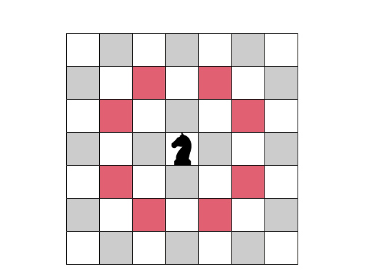
Exemple des 8 déplacements possibles du cavalier
Il s'agit d'un problème combinatoire qui demande beaucoup de calculs car il faut tester tous les cas possibles pour trouver une, voire toutes les solutions. Ce problème est en effet NP-Complet.
9.2. Version mono-thread
Voici le code de la version séquentielle, pour lequel on commence la résolution en position $(0,0)$, coin haut gauche sur l'échiquier.
- CODE
- knight_mono.cpp
- /**
- * Author: Jean-Michel Richer
- * Date: September 2025
- *
- * Resolution of the Knight's Tour problem which consist in finding
- * a hamiltonian path that visits each cell of a chessboard of size NxN
- * only once.
- *
- *
- * Results on AMD Ryzen 5 9600X
- * N #Solutions Time(s)
- * 4 0 0.002 s
- * 5 304 0.022 s
- * 6 524488 165.809 s
- */
- #include <iostream>
- #include <iomanip>
- #include <vector>
- #include <cstring>
- #include <cstdint>
- using namespace std;
- #include <getopt.h>
- string b_green = "\033[32m";
- string e_green = "\033[0m";
- string b_red = "\033[31m";
- string e_red = "\033[0m";
- // chessboard dimension (N)
- int dimension = 5;
- // number of solutions found
- uint64_t nbr_solutions = 0;
- /**
- * Class represents a coordinate on the chessboard
- */
- class Coordinate {
- public:
- int y, x;
- /**
- * Default constructor
- */
- Coordinate() {
- y = x = 0;
- }
- /**
- * Constructor from coorindate y and x
- */
- Coordinate( int _y, int _x) {
- y = _y;
- x = _x;
- }
- /**
- * Copy constructor
- */
- Coordinate(const Coordinate& obj) {
- y = obj.y;
- x = obj.x;
- }
- /**
- * Overloading of assignment operator
- */
- Coordinate& operator=(const Coordinate& obj) {
- if (this != &obj) {
- y = obj.y;
- x = obj.x;
- }
- return *this;
- }
- /**
- * Overloading of addition operator
- */
- Coordinate operator+(const Coordinate& rhs) const {
- return Coordinate(this->y + rhs.y, this->x + rhs.x);
- }
- /**
- * Overloading of output operator
- */
- friend ostream& operator<<(ostream& out, Coordinate& obj) {
- out << '(' << obj.y << ',' << obj.x << ')';
- return out;
- }
- };
- // ------------------------------------------------------------------
- // Definition of the moves of the knight from an initial position
- const int MAX_MOVES = 8;
- vector<Coordinate> moves = { Coordinate(1,2), Coordinate(2,1),
- Coordinate(2,-1), Coordinate(1,-2),
- Coordinate(-1,-2), Coordinate(-2,-1),
- Coordinate(-2,1), Coordinate(-1,2) };
- /**
- * Class that represents the chessboard
- */
- class Chessboard {
- public:
- static const int EMPTY = 0;
- // dimension of chessboard
- int dim;
- // size = dimension * dimension
- size_t size;
- // allocated array of data
- int *data;
- /**
- * Default constructor
- * @param rows number of rows or number of columns
- */
- Chessboard(int rows) {
- dim = rows;
- size = dim * dim;
- data = new int [ size ];
- for (size_t i = 0; i < size; ++i) {
- data[i] = EMPTY;
- }
- }
- /**
- * Copy constructor
- */
- Chessboard(Chessboard& obj) {
- dim = obj.dim;
- size = dim * dim;
- data = new int [ size ];
- memcpy(data, obj.data, sizeof(int) * size);
- }
- /**
- * Overloading of assignment operator
- */
- Chessboard& operator=(const Chessboard& obj) {
- if (&obj != this) {
- dim = obj.dim;
- size = dim * dim;
- memcpy(data, obj.data, sizeof(int) * size);
- }
- return *this;
- }
- /**
- * Overloading of operator [] to access a cell given
- * its coordinates
- */
- int& operator[](Coordinate& c) {
- return data[c.y * dim + c.x];
- }
- /**
- * Tells if coordinate c is inside [0,dimension-1]
- * and if cell of coordinate c is EMPTY
- */
- bool is_valid(Coordinate& c) {
- if ((0 <= c.x) and (0 <= c.y) and (c.x < dim) and (c.y < dim)) {
- return data[c.y * dim + c.x ] == EMPTY;
- } else {
- return false;
- }
- }
- /**
- * Overloading of output operator
- */
- friend ostream& operator<<(ostream& out, Chessboard& obj) {
- for (int y = 0; y < obj.dim; ++y) {
- for (int x = 0; x < obj.dim; ++x) {
- int value = obj.data[y * obj.dim + x] ;
- if (value == 1) {
- out << b_green << setw(4) << value << e_green;
- } else if (value == static_cast<int>(obj.size)) {
- out << b_red << setw(4) << value << e_red;
- } else {
- out << setw(4) << value;
- }
- out << ' ';
- }
- out << endl;
- }
- return out;
- }
- };
- /**
- * procedure used to recursively solve the problem.
- * Given a chessboard 'board' and a coordinate 'c' and the 'iteration'
- * we try to move the knight from 'c' to another valid position and
- * continue the search until we have visited all the cells
- */
- void solve(Chessboard& board, Coordinate c, int iteration) {
- if (iteration == static_cast<int>(board.size)) {
- // we have visited all the cells, so we have a new solution
- board[c] = iteration;
- ++nbr_solutions;
- if (nbr_solutions == 1) {
- cout << board << endl;
- }
- board[c] = Chessboard::EMPTY;
- } else {
- // otherwise try to move the knight to another cell
- // that has not been visited
- board[c] = iteration;
- for (auto m : moves) {
- Coordinate d = c + m;
- if (board.is_valid(d)) {
- //cout << "goto " << d << endl;
- //cout << board << endl << endl;
- solve(board, d, iteration+1);
- }
- }
- board[c] = Chessboard::EMPTY;
- }
- }
- /**
- * Main function
- */
- int main(int argc, char *argv[]) {
- int opt;
- while ((opt = getopt(argc, argv, "n:")) != -1) {
- switch (opt) {
- case 'n':
- dimension = std::stoi(optarg);
- break;
- default: /* '?' */
- cerr << "Usage: " << argv[0] << "[-n dimension]" << endl;
- exit(EXIT_FAILURE);
- }
- }
- // create chessboard
- Chessboard chessboard(dimension);
- // start from this position to find paths
- Coordinate top_left(0,0);
- // find the hamiltonian paths
- solve(chessboard, top_left, 1);
- // report number of paths found
- cout << "nbr_solutions=" << nbr_solutions << endl;
- return EXIT_SUCCESS;
- }
Ce programme accepte un paramètre en ligne de commadne introduit par
Afin de gérer au mieux le problème, on définit deux classes :
Coordinate : qui permet de gérer les coordonnées de déplacement du cavalier, cette classe est dotée de deux composantes entièresy etet on a également redéfini l'opérateur d'addition Chessboard qui gère l'échiquier de dimensiondim sous forme d'un tableau à une dimension de $dim × dim$ entiers
Etudiez le code, notamment la méthode solve, puis le compiler et déterminer le temps d'exécution pour des dimensions de l'échiquier de 4, 5 et 6.
| dimension | Solutions | Temps(s) |
| 4 | 0 | 0.002 |
| 5 | 304 | 0.019 |
| 6 | 524486 | 168.226 |
9.3. Version parallèle OpenMP
On désire créer une version parallèle pour résoudre ce problème en se basant sur des Tasks OpenMP.
Créer un nouveau fichier
On procède ainsi :
- dans un premier temps on crée les différents échiquiers qui correspondent à la résolution sur une profondeur donnée, on garde également la dernière coordonnée à remplir
- dans un second temps on lance la résolution du problème en créant une tâche pour chaque échiquier à résoudre
9.3.1. Calcul des échiquier et coordonnées
Par exemple dans le cas où la dimension est 5 et avec une profondeur de 3, on obtient 10 échiquiers différents. Par exemple, pour le premier échiquier, la troisième itération de la résolution consistera à placer le cavalier en position $(y=2,x=4)$.
--------------
   1    0    0    0    0    0
   0    0    2    0    0    0
   0    0    0    0    3    0
   0    0    0    0    0    0
   0    0    0    0    0    0
   0    0    0    0    0    0
(2,4)

--------------
   1    0    0    0    0    0
   0    0    2    0    0    0
   0    0    0    0    0    0
   0    0    0    3    0    0
   0    0    0    0    0    0
   0    0    0    0    0    0
(3,3)

--------------
   1    0    0    0    0    0
   0    0    2    0    0    0
   0    0    0    0    0    0
   0    3    0    0    0    0
   0    0    0    0    0    0
   0    0    0    0    0    0
(3,1)

--------------
   1    0    0    0    0    0
   0    0    2    0    0    0
   3    0    0    0    0    0
   0    0    0    0    0    0
   0    0    0    0    0    0
   0    0    0    0    0    0
(2,0)

--------------
   1    0    0    0    3    0
   0    0    2    0    0    0
   0    0    0    0    0    0
   0    0    0    0    0    0
   0    0    0    0    0    0
   0    0    0    0    0    0
(0,4)

--------------
   1    0    0    0    0    0
   0    0    0    0    0    0
   0    2    0    0    0    0
   0    0    0    3    0    0
   0    0    0    0    0    0
   0    0    0    0    0    0
(3,3)

--------------
   1    0    0    0    0    0
   0    0    0    0    0    0
   0    2    0    0    0    0
   0    0    0    0    0    0
   0    0    3    0    0    0
   0    0    0    0    0    0
(4,2)

--------------
   1    0    0    0    0    0
   0    0    0    0    0    0
   0    2    0    0    0    0
   0    0    0    0    0    0
   3    0    0    0    0    0
   0    0    0    0    0    0
(4,0)

--------------
   1    0    3    0    0    0
   0    0    0    0    0    0
   0    2    0    0    0    0
   0    0    0    0    0    0
   0    0    0    0    0    0
   0    0    0    0    0    0
(0,2)

--------------
   1    0    0    0    0    0
   0    0    0    3    0    0
   0    2    0    0    0    0
   0    0    0    0    0    0
   0    0    0    0    0    0
   0    0    0    0    0    0
(1,3)
9.3.2. Résultats
Calculer le temps d'exécution pour une dimension de 6 et une profondeur de 4 pour laquelle il ya 44 échiquiers différents. Faire varier le nombre de threads de 2 à 20 par pas de 2.
| dimension | Solutions | Tâches/thread | Temps(s) |
| 2 | 524486 | 22 | 92.34 |
| 4 | 524486 | 11 | 51.21 |
| 6 | 524486 | 8 | 37.56 |
| 8 | 524486 | 6 | 37.85 |
| 10 | 524486 | 5 | 35.57 |
| 12 | 524486 | 4 | 32.74 |
| 14 | 524486 | 4 | 33.06 |
| 16 | 524486 | 3 | 32.80 |
| 18 | 524486 | 3 | 32.81 |
| 20 | 524486 | 3 | 32.73 |
Par exemple avec une dimension de l'échiquier de 6 et une profondeur de 4, si on a recrours à 8 threads pour résoudre le problème sur AMD Ryzen 5 9600X, on obtient :
export OMP_NUM_THREADS=8 && /usr/bin/time -f "execution_time=%e" ./knight_omp_tasks.exe -n 6 -m 4

there are 44 tasks to execute

- task 0 : 8.46859 seconds for thread 6
- task 1 : 5.7393 seconds for thread 7
- task 2 : 3.50401 seconds for thread 0
- task 3 : 5.00047 seconds for thread 1
- task 4 : 5.15148 seconds for thread 2
- task 5 : 2.05625 seconds for thread 4
- task 6 : 1.94991 seconds for thread 5
- task 7 : 1.76351 seconds for thread 3
- task 8 : 1.75119 seconds for thread 3
- task 9 : 1.49845 seconds for thread 5
- task 10 : 1.46311 seconds for thread 4
- task 11 : 1.52257 seconds for thread 5
- task 12 : 5.77652 seconds for thread 0
- task 13 : 5.58854 seconds for thread 3
- task 14 : 3.30222 seconds for thread 4
- task 15 : 5.17749 seconds for thread 5
- task 16 : 2.28995 seconds for thread 1
- task 17 : 7.84392 seconds for thread 2
- task 18 : 18.442 seconds for thread 7
- task 19 : 11.1514 seconds for thread 4
- task 20 : 19.8327 seconds for thread 1
- task 21 : 15.804 seconds for thread 6
- task 22 : 1.91076 seconds for thread 3
- task 23 : 3.06135 seconds for thread 0
- task 24 : 1.5603 seconds for thread 5
- task 25 : 1.61171 seconds for thread 3
- task 26 : 1.26413 seconds for thread 5
- task 27 : 2.57747 seconds for thread 0
- task 28 : 1.58449 seconds for thread 3
- task 29 : 5.12105 seconds for thread 5
- task 30 : 5.3464 seconds for thread 2
- task 31 : 5.16721 seconds for thread 3
- task 32 : 3.01771 seconds for thread 0
- task 33 : 5.96769 seconds for thread 0
- task 34 : 18.367 seconds for thread 4
- task 35 : 9.65327 seconds for thread 5
- task 36 : 15.0508 seconds for thread 2
- task 37 : 4.55982 seconds for thread 3
- task 38 : 10.6651 seconds for thread 0
- task 39 : 5.26104 seconds for thread 3
- task 40 : 5.374 seconds for thread 7
- task 41 : 3.23772 seconds for thread 6
- task 42 : 4.72301 seconds for thread 1
- task 43 : 3.05638 seconds for thread 6
====================
thread 0: 34.5698 s
thread 1: 31.8461 s
thread 2: 33.3925 s
thread 3: 29.1983 s
thread 4: 36.34 s
thread 5: 27.7472 s
thread 6: 30.5667 s
thread 7: 29.5553 s
max_depth=4
nbr_boards=44
nbr_solutions=524486

execution_time=36.34
En fonction de la répartition des tâches sur les threads on aura un temps de calcul qui varie quelque peu entre 35.38s et 39.49s (tests réalisés sur 10 exécutions).
9.3.3. Equilibrage de charge
Si on connait la durée des 44 tâches, comment faire pour trouver la meilleure répartition possible sur $N$ threads ?
Trouver la meilleure répartition de tâches sur N dispositifs d'exécution est un problème d'équilibrage de charge (Load balancing), qui relève de la théorie de l'ordonnancement. C'est un problème NP-difficile, ce qui signifie qu'il n'existe pas d'algorithme polynomial pour trouver la solution optimale de manière exacte. Par conséquent, on utilise généralement des heuristiques ou des algorithmes d'approximation.
Un algorithme de traitement du problème est celui du Bin-Packing. Il consiste en deux étapes :
- trier les tâches par ordre décroissant de leur temps d'exécution
- pour chaque tâche, la placer sur le dispositif qui a actuellement la charge de travail totale la plus faible
Le résultat obtenu avec les 44 tâches suivantes et 8 threads est de 32.7694 s :
5.63733,5.82898,2.13803,7.57873,3.57109,3.40325,2.8873,1.64923,
1.73224,1.44767,2.63834,1.8494,5.7258,5.56542,3.25767,5.00461,
3.64545,5.19549,18.1034,11.0291,27.4202,15.4509,1.92096,3.09143,
1.64978,1.69641,1.22355,1.60807,2.62055,5.31367,3.41655,4.98055,
3.03668,3.34648,17.8144,9.65983,14.7994,5.54734,11.2256,7.28217,
3.58671,3.21031,4.63206,2.90992
Implantez cet algorithme en C++ ou en Python.
9.4. Version parallèle MPI
Sur le même principe que précédemment créer une version parallèle utilisant MPI.
Créer un nouveau fichier
Exécuter le programme en utilisant plusieurs processus : de 2 à 12 par pas de 2 par exemple.
9.4.1. Execution sur une machine
Exécution sur AMD Ryzen 5 9600X.
Temps de référence (1 thread): 175.1500 s

================================================================================
Analyse de la performance de l'application
Fraction parallèle (Par) utilisée pour Amdahl: 0.99
================================================================================
Threads    | Temps (s)    | Accélération    | Amdahl          | Karp-Flatt
--------------------------------------------------------------------------------
1          | 175.1500     | 1.0000          | 1.0000          | -1.0000
2          | 89.6200      | 1.9544          | 1.9802          | 0.0234
4          | 66.8500      | 2.6200          | 3.8835          | 0.1756
6          | 52.6300      | 3.3279          | 5.7143          | 0.1606
8          | 49.6500      | 3.5277          | 7.4766          | 0.1811
10         | 35.5900      | 4.9213          | 9.1743          | 0.1147
12         | 34.3300      | 5.1020          | 10.8108         | 0.1229

================================================================================
 1  -----  -----
 2 -48.83 -48.83
 4 -61.83 -13.00
 6 -69.95  -8.12
 8 -71.65  -1.70
10 -79.68  -8.03
12 -80.40  -0.72
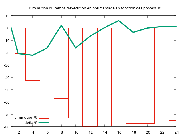
9.4.2. Execution sur deux machines
On réalise les tests sur deux machines :
- AMD Ryzen 5 9600X à 5,4 GHz, 12 threads
- AMD Ryzen 5 5600G à 4,4 GHz, 12 threads
On répartit équitablement les processus sur les deux machines en allant de 2 à 24 threads par pas de 2.
Temps de référence (1 thread): 175.1500 s

================================================================================
Analyse de la performance de l'application
Fraction parallèle (Par) utilisée pour Amdahl: 0.99
================================================================================
Threads    | Temps (s)    | Accélération    | Amdahl          | Karp-Flatt
--------------------------------------------------------------------------------
1          | 175.1500     | 1.0000          | 1.0000          | -1.0000
2          | 138.8200     | 1.2617          | 1.9802          | 0.5852
4          | 100.2000     | 1.7480          | 3.8835          | 0.4294
6          | 71.6500      | 2.4445          | 5.7143          | 0.2909
8          | 75.4400      | 2.3217          | 7.4766          | 0.3494
10         | 47.2400      | 3.7077          | 9.1743          | 0.1886
12         | 35.5200      | 4.9310          | 10.8108         | 0.1303
14         | 35.8600      | 4.8843          | 12.3894         | 0.1436
16         | 46.2100      | 3.7903          | 13.9130         | 0.2148
18         | 40.0300      | 4.3755          | 15.3846         | 0.1832
20         | 39.9300      | 4.3864          | 16.8067         | 0.1873
22         | 41.9000      | 4.1802          | 18.1818         | 0.2030
24         | 43.5400      | 4.0227          | 19.5122         | 0.2159

================================================================================
 1  -----  -----
 2 -20.74 -20.74
 4 -42.79 -22.05
 6 -59.09 -16.30
 8 -56.93   2.16
10 -73.03 -16.10
12 -79.72  -6.69
14 -79.53   0.19
16 -73.62   5.91
18 -77.15  -3.53
20 -77.20  -0.06
22 -76.08   1.12
24 -75.14   0.94