1. Introduction au C++
1.11. Débogage, profilage, optimisation
Le processus de développement d'un programme passe par trois étapes
- le débogage consiste à éliminer les erreurs qui font planter/crasher le programme ou qui conduisent à des résultats erronés
- le profilage a pour but de déterminer quels sont les parties du code qui nécessitent d'être améliorées car elles consomment beaucoup de temps CPU (hot spot)
- l'optimisation vise à donner une réponse au profilage
1.11.1. Débogage
1.11.1.a Electric Fence
Electric Fence helps you detect two common programming bugs:
- software that overruns the boundaries of a malloc() memory allocation,
- software that touches a memory allocation that has been released by free().
- Unlike other malloc() debuggers, Electric Fence will detect read accesses as well as writes, and it will pinpoint the exact instruction that causes an error.
Installer le paquet Electric-Fence qui permet de traquer les erreurs d'accès à la mémoire :
sudo apt-get install electric-fenceCompiler ensuite le programme en réalisant l'édition de liens avec Electric Fence :
- CODE
- efence.c
gcc -c efence.c -ggdb
gcc -o efence.exe efence.o -ggdb -lefence
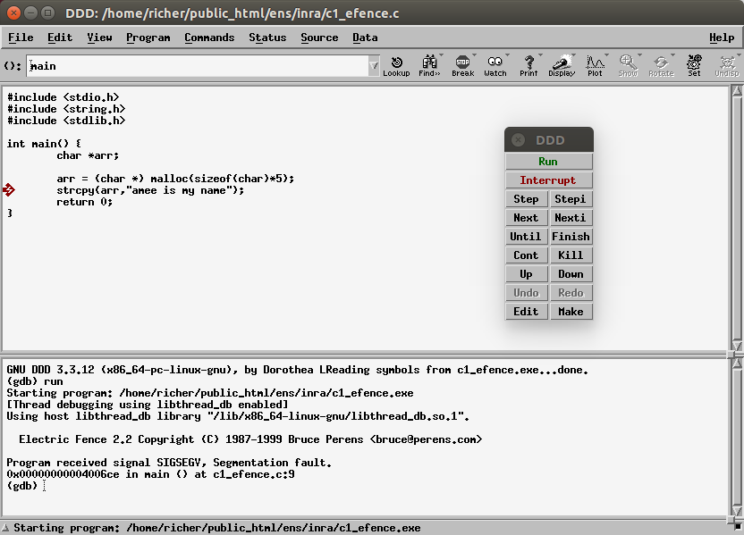
1.11.1.b Utilisation d'un débogueur
Il existe plusieurs débogueurs sous Linux :
- gdb : en ligne de commande
- xxgdb : version graphique X11 de gdb
- ddd (Data Display Debugger) version graphique plus facile à utiliser
Compiler ensuite le programme avec -ggdb :
gcc -o my.exe my_program.o -ggdb
Puis lancer ddd sur l'exécutable :
ddd my.exe
1.11.2. Profilage
Dans la suite de cette section, nous étudions le comportement du programme suivant :
- CODE
- proc.c
- /* ===================================================
- * compile with gcc :
- * gcc -pg -o prog.exe prog.c
- * ./prog.exe
- * gprof prog.exe
- * =================================================== */
- #include <stdio.h>
- #include <stdlib.h>
- #include <time.h>
- // number of loops for each calculation
- #define MAX_LOOPS 2000
- // first dimension of arrays (number of rows)
- #define SIZE1 1000
- // second dimension of arrays (number of columns)
- #define SIZE2 2000
- // type of array
- #define TYPE float
- /**
- * allocate matrix of size : SIZE1*SIZE2*sizeof(TYPE)
- */
- TYPE **allocate_array() {
- int i;
- TYPE **array;
- for (i=0;i<SIZE1;++i) {
- }
- return array;
- }
- /**
- * fill matrix with random values
- */
- void fill_array(TYPE **a) {
- int i, j;
- for (i=0;i<SIZE1;++i) {
- for (j=0;j<SIZE2;++j) {
- }
- }
- }
- /**
- * function that is called
- * MAX_LOOPS * SIZE1 / 2 times by proc21
- * MAX_LOOPS * SIZE1 / 2 times by proc21
- *
- */
- void proc3(TYPE *c, TYPE *a, TYPE *b, int k) {
- int j;
- for (j=0;j<SIZE2;++j) {
- c[j]=a[j]*k+b[j];
- }
- }
- /**
- * first calculation
- */
- void proc21(TYPE **a, TYPE **b) {
- int i;
- for (i=0;i<SIZE1;i+=2) {
- proc3(a[i+1],a[i],b[i],3);
- }
- }
- /**
- * second calculation
- */
- void proc22(TYPE **a, TYPE **b) {
- int i;
- for (i=0;i<SIZE1;i+=2) {
- proc3(b[i+1],a[i],b[i],-5);
- }
- }
- /**
- * function that calls
- * MAX_LOOPS times proc21
- * MAX_LOOPS times proc22
- */
- void proc1(TYPE **a, TYPE **b) {
- int i;
- for (i=0; i<MAX_LOOPS; ++i)
- proc21(a,b);
- for (i=0; i<MAX_LOOPS; ++i)
- proc22(a,b);
- }
- int main() {
- TYPE **a1, **a2;
- // allocate matrices
- a1 = allocate_array();
- a2 = allocate_array();
- // fill matrices
- fill_array(a1);
- fill_array(a2);
- // call main function for computations
- proc1(a1,a2);
- return 0;
- }
1.11.2.a Utilisation de prof/gprof sous Unix
On utilse les options de compilation classiques avec gprof :
> gcc -o prog.exe prog.c -pg
> ./prog.exe
> gprof prog.exe >prog_gprof.txt
Le résultat en sortie peut être visualisé ici.
a) profil à plat
Le flat profile est le suivant :
Flat profile:

Each sample counts as 0.01 seconds.
  %   cumulative   self              self     total
 time   seconds   seconds    calls   s/call   s/call  name
 99.55     21.94    21.94  2000000     0.00     0.00  proc3
  0.27     22.00     0.06        2     0.03     0.03  fill_array
  0.09     22.02     0.02     2000     0.00     0.01  proc21
  0.09     22.04     0.02     2000     0.00     0.01  proc22
  0.00     22.04     0.00        2     0.00     0.00  allocate_array
  0.00     22.04     0.00        1     0.00    21.98  proc1
On peut donc lire que :
- le sous-programme proc3 a été appelé 2.000.000 de fois et a consommé 99.55% du temps CPU (soit 21.94s sur les 22.04s du temps d'exécution total), c'est donc cette fonction qu'il faudra optimiser
- proc21 a été appelé 2000 fois, ainsi que proc22 : bien que proc21 et proc22 appellent proc3, ici n'est reporté que le temps d'exécution hors appels aux autres sous-programmes.
b) granularité
Le second type d'information reporté par gprof concerne la granularité, c'est à dire le temps total passé dans chaque sous-programme ainsi que le nombre d'appels aux autres sous-programmes :
index % time    self  children    called     name

[1]    100.0    0.00   22.04                 main [1]
                0.00   21.98       1/1           proc1 [2]
                0.06    0.00       2/2           fill_array [6]
                0.00    0.00       2/2           allocate_array [7]
-----------------------------------------------
                0.00   21.98       1/1           main [1]
[2]     99.7    0.00   21.98       1         proc1 [2]
                0.02   10.97    2000/2000        proc21 [4]
                0.02   10.97    2000/2000        proc22 [5]
-----------------------------------------------
               10.97    0.00 1000000/2000000     proc21 [4]
               10.97    0.00 1000000/2000000     proc22 [5]
[3]     99.5   21.94    0.00 2000000         proc3 [3]
-----------------------------------------------
                0.02   10.97    2000/2000        proc1 [2]
[4]     49.9    0.02   10.97    2000         proc21 [4]
               10.97    0.00 1000000/2000000     proc3 [3]
-----------------------------------------------
                0.02   10.97    2000/2000        proc1 [2]
[5]     49.9    0.02   10.97    2000         proc22 [5]
               10.97    0.00 1000000/2000000     proc3 [3]
-----------------------------------------------
                0.06    0.00       2/2           main [1]
[6]      0.3    0.06    0.00       2         fill_array [6]
-----------------------------------------------
                0.00    0.00       2/2           main [1]
[7]      0.0    0.00    0.00       2         allocate_array [7]
-----------------------------------------------
On voit donc que :
- [1] la fonction main consomme 100% du temps d'exécution, ce qui est normal puisque c'est elle qui se trouve au sommet de l'arbre d'appel des sous-programmes.
- [2] c'est ensuite au tour de proc1 d'appeler :
- proc21 : 2000 fois, soit 10.97s
- proc22 : 2000 fois, soit 10.97s
- [3] proc3 est appelé 2.000.000 de fois :
- 1.000.000 de fois par proc21
- 1.000.000 de fois par proc22
1.11.2.b Utilisation de VTune Analyzer (Intel)
VTune est un outil complet de profiling et de tuning qui permet de déterminer les hot spots et d'éclairer sur leur comportement : instruction peu performante, accès mémoire non aligné, nombre important de défauts de cache dus à des données de trop grande taille.
1.11.2.c cas de prog.c
- Call Graph Wizard
- Sampling Wizard (% utilisation par sous-programme)
- Sampling Wizard (proc3, code source)
- Sampling Wizard (proc3, code source et assembleur)
1.11.2.d Utilisation de Valgrind
valgrind est un ensemble d'utilitaires qui servent à débuguer et profiler les programmes
Valgrind is an instrumentation framework for building dynamic analysis tools. There are Valgrind tools that can automatically detect many memory management and threading bugs, and profile your programs in detail. You can also use Valgrind to build new tools.
The Valgrind distribution currently includes six production-quality tools:
- a memory error detector (--tool=memcheck)
- two thread error detectors (--tool=helgrind)
- a cache and branch-prediction profiler (--tool=cachegrind)
- a call-graph generating cache and branch-prediction profiler (--tool=callgrind)
- a heap profiler (--tool=massif)
- a tool for detecting errors in multithreaded C and C++ programs (--tool=drd)
It also includes three experimental tools: a stack/global array overrun detector, a second heap profiler that examines how heap blocks are used, and a SimPoint basic block vector generator
Voir également dans la partie C++11 l'utilisation de valgrind avec l'outil memcheck ainsi que ce tutoriel.
On compile le programme à étudier avec l'option de débugage -g puis il suffit de lancer le profilage. Attention cependant car certaines options peuvent augmenter le temps d'exécution d'un facteur 20 à 100 par rapport à une exécution normale.
Dans le cas de l'outil callgrind (équivalent de gprof), on tapera au niveau du shell :
valgrind --tool=callgrind --dump-instr=yes --simulate-cache=yes --collect-jumps=yes <executable> [args...]Les options --dump-instr=yes --simulate-cache=yes ou --collect-jumps=yes peuvent être supprimées afin de gagner du temps.
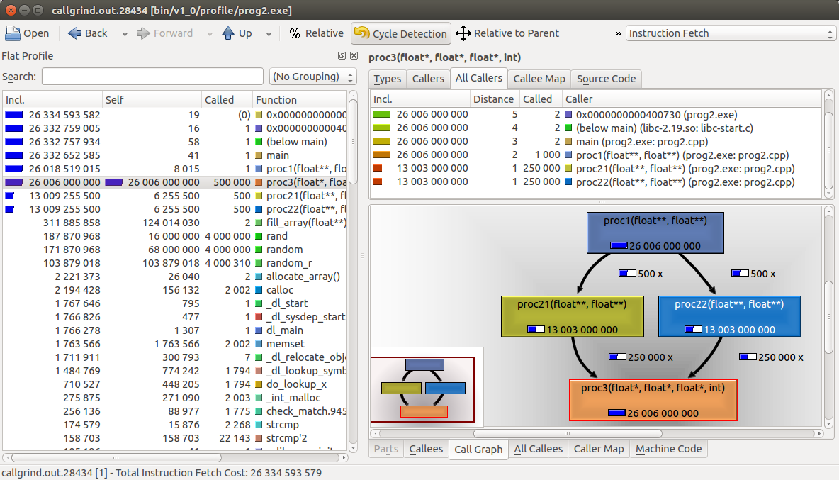
Utilisation de kcachegrind pour visualiser les résultats
en sortie de valgrind
Pour obtenir le visuel du call-graph (il faut avoir installé graphviz -- graph visualization software -- sous Ubuntu : sudo apt-get install graphviz), il suffit de cliquer en bas à droite sur l'onglet "Call-graph".
Si seule une partie du code vous intéresse, vous pouvez faire en sorte que valgrind ne se déclenche qu'à partir de l'appel d'un sous-programme, comme sur l'exemple suivant :
- #include <valgrind/callgrind.h>
- int main() {
- code_with_no_instrumentation();
- CALLGRIND_START_INSTRUMENTATION;
- CALLGRIND_TOGGLE_COLLECT;
- code_to_analyze();
- CALLGRIND_TOGGLE_COLLECT;
- CALLGRIND_STOP_INSTRUMENTATION;
- code_with_no_instrumentation();
- exit(EXIT_SUCCESS);
- }
Il faudra alors relancer valgrind avec les options --collect-at-start=no et --instru-at-start=no :
valgrind --tool=callgrind --dump-instr=yes --simulate-cache=yes --collect-jumps=yes --collect-at-start=no --instru-at-start=no <executable> [args...]1.11.3. Optimisation
L'optimisation est parfois difficile à réaliser et demande beaucoup d'efforts afin d'améliorer sensiblement le code (cf. Cours L3 Informatique). Certaines techniques sont à utiliser :
- dépliage de boucle
- tuilage (loop tiling)
- allocation par bloc
- utilisation de librairies dédiées et optimisées (cf. Librairies dédiées au calcul scientifique)
Cependant, les options de compilation des compilateurs permettent parfois d'obtenir un gain substantiel. Par exemple sous gcc/c++ :
- -ftree-vectorize -ftree-vectorizer-verbose=1 -msse4.2 : vectorisation du code avec SSE4.2
- -ftree-vectorize -ftree-vectorizer-verbose=1 -mavx2 : vectorisation du code avec AVX2
- -funroll-loops --param max-unroll-times=4 : dépliage des boucles
Sous Linux, pour connaître les différentes technologies disponibles sur un processeur il suffit de taper la commande suivante :
cat /proc/cpuinfo | grep "model name" | uniq ; cat /proc/cpuinfo | grep -E "flags" | uniqVoici un exemple de sortie pour un processeur Intel Xeon E5-2670 v2 (Q3'13, 10 cores + 10 threads, 25 Mo L3, Turbo Freq. 3.3 Ghz, \$1550) :
model name	: Intel(R) Xeon(R) CPU E5-2670 v2 @ 2.50GHz
flags		: fpu vme de pse tsc msr pae mce cx8 apic sep mtrr pge mca cmov pat pse36 clflush dts acpi mmx fxsr sse sse2 ss ht tm pbe syscall nx pdpe1gb rdtscp lm constant_tsc arch_perfmon pebs bts rep_good xtopology nonstop_tsc aperfmperf pni pclmulqdq dtes64 monitor ds_cpl vmx smx est tm2 ssse3 cx16 xtpr pdcm pcid dca sse4_1 sse4_2 x2apic popcnt tsc_deadline_timer aes xsave avx f16c rdrand lahf_lm ida arat xsaveopt pln pts dts tpr_shadow vnmi flexpriority ept vpid fsgsbase smep erms