Ce site est en cours de reconstruction certains liens peuvent ne pas fonctionner ou certaines images peuvent ne pas s'afficher.
11.1. Linear Regression
Consider three series of data that we want to compare, we want to know if the data of $x$ are related to $y$ or $z$ via a linear relationship.
> x <- c(10,20,30,40,50)
> y <- c(105, 210, 302, 415, 506)
> z <- c(10,60,80,40,25)
By plotting y and z in function of $x$ we can see that there exists a linear relationship between $x$ and $y$ but not between $x$ and $z$.
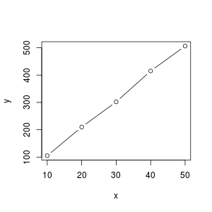
y = f(x), linear
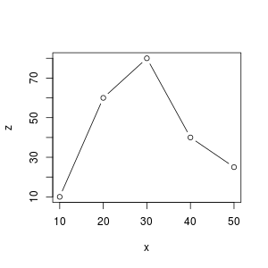
z = f(x), parabola
In order to confirm the linear relationship between $x$ and $y$ we could use the cor() function or R.
The correlation coefficient of two variables in a data set equals to their covariance divided by the product of their individual standard deviations. It is a normalized measurement of how the two are linearly related.
If the correlation coefficient is close to 1, it would indicate that the variables are positively linearly related
> cor(x,y)               # x and y are strongly related (value close to 1.0)
[1] 0.9995255
> cor(x,z)
[1] 0.05698029           # x and z are not related linearly (value close to 0.0)
Simple linear regression
Let us determine if $x$ is related to $y$, by performing a linear regression that will try to find a formula to predict $x$ from $y$ of the form $x' = c_0 + c_1 × y + ε$, where $ε$ is some residual error:
lm is used to fit linear models. It can be used to carry out regression, single stratum analysis of variance and analysis of covariance (although ‘aov’ may provide a more convenient interface for these).
> x <- c(10,20,30,40,50)
> y <- c(105, 210, 302, 415, 506)
> z <- c(60, 16, 1, 18, 64)
# apply linear regression
> fit <- lm(y ~ x)
> summary(fit)
/*
Call:
lm(formula = y ~ x)

Residuals:
   1    2    3    4    5
-1.2  3.1 -5.6  6.7 -3.0

Coefficients:
            Estimate Std. Error t value Pr(>|t|)
(Intercept)   5.5000     5.9422   0.926    0.423
x            10.0700     0.1792  56.205 1.24e-05 ***
---
Signif. codes:  0 ‘***’ 0.001 ‘**’ 0.01 ‘*’ 0.05 ‘.’ 0.1 ‘ ’ 1

Residual standard error: 5.666 on 3 degrees of freedom
Multiple R-squared:  0.9991,	Adjusted R-squared:  0.9987
F-statistic:  3159 on 1 and 3 DF,  p-value: 1.241e-05
*/
> fit$fitted.values
    1     2     3     4     5
106.2 206.9 307.6 408.3 509.0
From the previous calculation we see that the p-value is close to 0 (1.241e-05) and the $R^2$ value is close to 1.0 (0.9991 ) which means that the data are correlated by a linear relation.
The p-value helps you determine the significance of your results, it is a probability (between 0 and 1.0) that the difference observed between data is due to randomness. In other words:
- if the p-value is less than a threshold $α$ (generally 5%), so if $p < α = 0.05$, it is said that you reject the null hypothesis $H_0$, in plain language terms the null hypothesis is usually an hypothesis of no difference, so you accept the alternative hypothesis $H_1$ which is the opposite of the null hypothesis
- if $p > α$ then you can consider that the data are not related
By obtaining the coefficients (see below) we can determine that $y = 5.50 + 10.07 * x$.
> c = coefficients(fit)
> c
(Intercept)           x
       5.50       10.07

# define function f
>  f <- function(x) {
+ return (5.50 + 10.07 * x)
+ }
# apply function f to each element of x
> estimated_y = sapply(x, f)
> estimated_y
[1] 106.2 206.9 307.6 408.3 509.0
> abs(estimated_y - y)
[1]  9.8 14.1  5.4 17.7  8.0
> abs(estimated_y - y)/y
[1] 0.011428571 0.014761905 0.018543046 0.016144578 0.005928854
Finally the formula $f$ gives use values close to the ones of $x$.
For example for the first value $x=10$ we have $y=105$ and the estimated value of $y$ using $f(x)$ is 106.2, so this is a difference of $|106.2-105| = 1.2$ but only a 1.1% difference in the estimation.
If you apply the same reasoning between $z$ and $x$ then you will find:
> fit <- lm(z ~ x)
> summary(fit)
/*
Call:
lm(formula = z ~ x)

Residuals:
    1     2     3     4     5
 30.2 -14.8 -30.8 -14.8  30.2

Coefficients:
            Estimate Std. Error t value Pr(>|t|)
(Intercept)   28.800     34.312   0.839    0.463
x              0.100      1.034   0.097    0.929

Residual standard error: 32.71 on 3 degrees of freedom
Multiple R-squared:  0.003105,	Adjusted R-squared:  -0.3292
F-statistic: 0.009343 on 1 and 3 DF,  p-value: 0.9291
*/
Here the p-value is greater than 0.05 (0.9291) and $R^2$ is far from 1.0 (0.003105), so the data are not related by a linear function.
Multiple linear regression
Consider the following set of data (hwas.RData) that concerns 45 persons for which we have:
- the height in cm
- the weight in kg
- the age in years
- the sex: M(ale) or F(emale)
> mydata <- read.table("hwas.RData", header=T)
> head(mydata)
  height.cm weight.kg age.years sex
1       171        66        43   M
2       179        76        75   M
3       170        70        64   M
4       177        73        44   M
5       164        64        76   M
6       158        48        84   M
> tail(mydata)
   height.cm weight.kg age.years sex
40       169        60        53   F
41       142        47        41   F
42       132        40        73   F
43       179        71        44   F
44       158        56        54   F
45       160        58        49   F
The question we want to answer is: is there a relationship between the weight of a person and its height, age and sex ?
For this we will try to establish a linear regression with multiple variables called a Multiple Linear Regression. In this example the sex is a qualitative variable and must be transformed into a factor.
We are looking for a formula of the form:
$$weight = c_0 + c_1 × height + c_2 × age + c_3 × factor(sex)$$
> fit <- lm(weight.kg ~ height.cm + age.years + factor(sex), mydata)
> summary(fit)
/*
Call:
lm(formula = weight.kg ~ height.cm + age.years + factor(sex),
    data = mydata)

Residuals:
    Min      1Q  Median      3Q     Max
-8.9930 -2.3789  0.0152  2.4916 10.6506

Coefficients:
              Estimate Std. Error t value Pr(>|t|)
(Intercept)  -49.79115    7.18988  -6.925  2.1e-08 ***
height.cm      0.67519    0.03940  17.138  < 2e-16 ***
age.years     -0.03552    0.03597  -0.988   0.3291
factor(sex)M   3.08788    1.20561   2.561   0.0142 *
---
Signif. codes:  0 ‘***’ 0.001 ‘**’ 0.01 ‘*’ 0.05 ‘.’ 0.1 ‘ ’ 1

Residual standard error: 3.899 on 41 degrees of freedom
Multiple R-squared:  0.8933,	Adjusted R-squared:  0.8855
F-statistic: 114.4 on 3 and 41 DF,  p-value: < 2.2e-16
*/
The summary of the model tells us that
- $c_0 = -49.79$ and $c_1 = 0.67$ have high significance
- the sex has a relatively low significance
- the age has no significance
We can obtain more information by plotting the fit:
png("plot_mlr.png", width=600, height=600)
layout(matrix(c(1,2,3,4),2,2))
plot(fit)
dev.off()
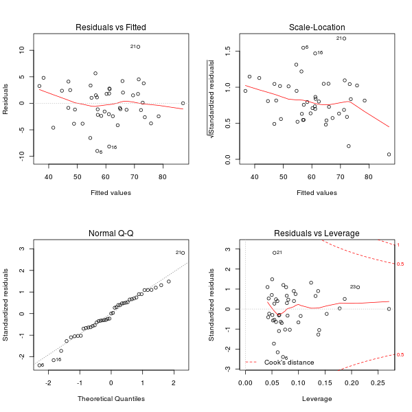
We can see that the rows 6, 16 and 21 are special cases that could be eliminated to get a better quality of the results. Indeed if you compute the following:
> abs(mydata$weight.kg - fitted(fit)) / mydata$weight.kg
           1            2            3            4            5            6
0.0185895122 0.0593196479 0.0599180243 0.0240749166 0.0417450186 0.1873539680
           7            8            9           10           11           12
0.0001746786 0.0856648324 0.0202647057 0.1244780636 0.0192085184 0.0137794968
          13           14           15           16           17           18
0.0434182144 0.0285949603 0.0323257050 0.1537868846 0.0424802727 0.0267483668
          19           20           21           22           23           24
0.0910796105 0.0296565849 0.1298858838 0.0369519727 0.0489174598 0.0187958505
          25           26           27           28           29           30
0.0394608419 0.1116779434 0.0803081176 0.0577353400 0.0245524695 0.0347036671
          31           32           33           34           35           36
0.1363442466 0.0498313711 0.0527068355 0.0016231839 0.0800729522 0.0293002426
          37           38           39           40           41           42
0.0171666004 0.0689881522 0.0179873810 0.0405570195 0.0504353766 0.0814775486
          43           44           45
0.0210558261 0.0183786203 0.0258828757
You can see that the estimation compared to the real value have for:
- for item 6, a difference of 18.73%
- for item 16, a difference of 15.37%
- for item 21, a difference of 12.98%
If we remove those rows we could get a more accurate prediction:
Warning: Undefined variable $weight in /home/jeanmichel.richer/public_html/r_lr.php on line 422
Warning: Undefined variable $weight in /home/jeanmichel.richer/public_html/r_lr.php on line 422
# remove rows 6, 16 and 21 don't forget the ',' at the end
> mydata <- mydata[ -c(6,16,21), ]
> fit <- lm(weight.kg ~ height.cm + age.years + factor(sex), mydata)
> summary(fit)
/*
Call:
lm(formula = weight.kg ~ height.cm + age.years + factor(sex),
    data = mydata)

Residuals:
    Min      1Q  Median      3Q     Max
-6.7751 -2.1153  0.0418  2.1985  5.1966

Coefficients:
               Estimate Std. Error t value Pr(>|t|)
(Intercept)  -49.052178   5.609898  -8.744 1.24e-10 ***
height.cm      0.660163   0.030770  21.455  < 2e-16 ***
age.years     -0.007251   0.028596  -0.254  0.80119
factor(sex)M   3.334148   0.954162   3.494  0.00122 **
---
Signif. codes:  0 ‘***’ 0.001 ‘**’ 0.01 ‘*’ 0.05 ‘.’ 0.1 ‘ ’ 1

Residual standard error: 3.022 on 38 degrees of freedom
Multiple R-squared:  0.9328,	Adjusted R-squared:  0.9275
F-statistic: 175.8 on 3 and 38 DF,  p-value: < 2.2e-16
*/

> sort(abs(mydata.kg - fitted(fit)) / mydata.kg)
         34          14          37           1          39           7
0.001967183 0.003663395 0.011945637 0.013001642 0.013740261 0.017049186
         11          44          12          24           9          20
0.018756076 0.020320199 0.020855313 0.022422828 0.026523095 0.028207040
          4          30          45          43          29           5
0.029974826 0.030568475 0.030712876 0.031013854 0.031270727 0.031286479
         15          22          23          36          40          18
0.033585688 0.033622933 0.034386588 0.034519136 0.035518640 0.035654057
         32          33          25          28          13           2
0.037691907 0.038652727 0.045318996 0.046220846 0.047950935 0.053850411
         41           3          17          42          38          27
0.055452709 0.056490516 0.059040199 0.060998981 0.067439092 0.069220703
         35          19          26           8          31          10
0.075250248 0.083816526 0.095299486 0.100601652 0.141146898 0.157403217
11.1.1. Multiple non linear regression
nls determines the nonlinear (weighted) least-squares estimates of the parameters of a nonlinear model
If you want to use nls() you need to provide a formula, so you already have an idea of what you are looking for.
Suppose you have the following data:
> x
[1] 10 20 30 40 50
> z
[1] 60 16  1 18 64
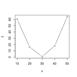
In this case the curve $z=f(x)$ looks like a parabola. So we will try to find a parabola of the form:
$$ a + b × (x - c)^2 $$ or $$ a'x^2 + b'x + c' $$
but we don't know the values of constants $a$, $b$ and $c$, so we need to provide values from where to start to the nls() function:
> fit <- nls(z ~ a*x^2+b*x+c, start=list(a=-100, b=-100,c=-100))
> summary(fit)
/*
Formula: z ~ a * x^2 + b * x + c

Parameters:
    Estimate Std. Error t value Pr(>|t|)
a   0.151429   0.001355   111.7 8.01e-05 ***
b  -8.985714   0.082882  -108.4 8.51e-05 ***
c 134.800000   1.087592   123.9 6.51e-05 ***
---
Signif. codes:  0 ‘***’ 0.001 ‘**’ 0.01 ‘*’ 0.05 ‘.’ 0.1 ‘ ’ 1

Residual standard error: 0.5071 on 2 degrees of freedom

Number of iterations to convergence: 1
Achieved convergence tolerance: 8.132e-09
*/
> coefficients(fit)
          a           b           c
  0.1514286  -8.9857143 134.8000000
> f <- function(x)  0.1514286*x^2-8.9857143*x+134.8
> sapply(x,f)
[1] 60.085717 15.657154  1.514311 17.657188 64.085785
> estimated_z <- sapply(x, f)
> estimated_z
[1] 60.085717 15.657154  1.514311 17.657188 64.085785
> abs(estimated_z - z)/z
[1] 0.001428617 0.021427875 0.514311000 0.019045111 0.001340391